22. Physically Based Shading
Chapter 10 gave us the Phong and Blinn–Phong models: a diffuse term, a highlight around the mirror direction, a sum over the lights.
Chapter 12 showed that the physical version of a "material" is the BRDF, that every surface turns into a mirror at grazing angles (Fresnel), and that a rough surface can be imagined as a landscape of tiny mirrors.
It also promised that Part 2 would put these pieces together properly.
That is this chapter.
Physically based shading (物理ベースシェーディング), the shading half of physically based rendering (PBR, 物理ベースレンダリング), is today's standard in film renderers, game engines and file formats like glTF.
It's not a single formula but a set of rules: measure light in physical units, use BRDFs that obey the laws of chapter 12, describe roughness with a microfacet model, and give artists a few parameters (base color, metallic, roughness) that can't produce impossible materials.
The payoff is consistency: a material made once looks right under the noon sun, in a dim room and in a reflection, without retuning.
Here's the plan:
- Radiometry, precisely (section 22.1): solid angle, flux, irradiance and radiance with the cosine factor, conversions with numbers, and photometry (lumens, nits) briefly.
- What a physical BRDF must do (22.2): the tests, Lambert passing them, Phong failing them.
- Microfacet theory (22.3): the Cook–Torrance formula derived, the GGX and Beckmann distributions, Smith's masking–shadowing, Fresnel with , and the roughness remapping.
- One light, fully worked (22.4), with C++ and shader code.
- The metallic–roughness workflow (22.5), the specular–glossiness workflow and glTF.
- Image-based lighting with PBR (22.6): irradiance from spherical harmonics, the split-sum approximation, and energy compensation.
- More layers (22.7): clear coat, sheen, anisotropy, subsurface.
- Area lights in real time (22.8): representative points and linearly transformed cosines.
This goes beyond the exam syllabus, but its foundations are exam topics: reflection models (反射モデル) from chapter 10 and the BRDF, Fresnel and microfacets of photorealistic rendering (写実的表現法) from chapter 12.
You need the radiometry and BRDF basics of chapter 12 (sections 12.2 to 12.4), linear color from chapter 3 (section 3.7), environment maps from chapter 11 (section 11.9), and the dot and cross products of Linear Algebra chapters 4 and 5.
A few integrals appear; as in chapter 12, I always say what they add up, and every one of them is checked numerically.
You'll implement all of this in the OpenGL series, chapter 24, and the sampling methods used to precompute some of it are the topic of chapter 23.
22.1 Radiometry, precisely
Chapter 12 introduced the four radiometric quantities with one table.
To build BRDFs we need them a bit more exactly, in particular where the cosine factors come from.
Solid angle in formulas
A direction above a surface is given by two angles: , measured from the normal (0 at the normal, at the horizon), and , the angle around the normal.
A tiny patch of directions with sides and cuts out of the unit sphere a little rectangle of height and width (the circle of latitude at has radius ), so its solid angle (立体角) is
With it, the two hemisphere integrals that keep coming back are easy:
A cone of half-angle around the normal covers steradians.
Worked example: the sun. The sun's disk has an angular radius of about 0.2666°, so it covers sr.
For small cones and the formula becomes (with in radians), the area of a small disk on the unit sphere: sr, the same.
Radiance and the cosine factor
Radiance (放射輝度) is power per area per solid angle, but the area is measured perpendicular to the ray, not along the surface:
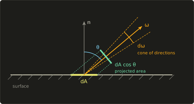
is the projected area (投影面積): how big the patch looks from direction .
That's why radiance is the quantity an eye or camera measures: a pixel sees a fixed solid angle and whatever area of surface fits into it.
And it explains the cosine in Lambert's law from both sides: light arriving at a slant is spread over a larger area ( per incoming direction), and light leaving at a slant comes from a projected area that shrinks with .
The other quantities follow by integrating:
| Quantity | Definition | Unit | Example |
|---|---|---|---|
| radiant flux (放射束) | total power | W | a lamp's whole output |
| radiant intensity (放射強度) | W/sr | a point light in one direction | |
| irradiance (放射照度) | W/m² | light arriving at a surface | |
| radiant exitance (放射発散度) | W/m² | light leaving a surface | |
| radiance (放射輝度) | W/(m²·sr) | light along one ray |
Worked conversions
An isotropic point light. A bulb radiates W evenly into the whole sphere of sr:
At m, a surface facing the light gets W/m²; tilted by 60° it gets half of that, 0.995 W/m².
A Lambertian emitter. A diffuse panel sends the same radiance in every direction of its hemisphere, so its exitance is (the same as chapter 12's uniform sky).
A 1 m² panel emitting 100 W therefore has
A small area light. Take a 0.25 m² piece of that panel, 2 m away, facing the receiver (), while the receiver is tilted by 30° ().
Seen from the receiver, the piece covers about sr, and all of that solid angle has radiance , so
This "radiance times solid angle times cosine" is only valid while the light is small compared with its distance; section 22.8 shows what happens when it isn't.
Why the sun is a directional light. On a clear day the sun delivers roughly 1000 W/m² to a surface facing it.
Spread over its sr, that's a radiance of about W/(m²·sr), hundreds of thousands of times that of the clear sky around it (a few tens of W/(m²·sr)).
A renderer that stored the sun inside an environment map would need to hit that tiny disk with its samples; it's far better to treat the sun as a directional light with a given irradiance, and the sky as the environment.
Photometry, briefly
The photometric quantities of chapter 3 are the same five ideas, each wavelength weighted by the eye's sensitivity (chapter 3's luminous efficiency curve), with the conversion factor 683 lm/W at 555 nm, where the eye is most sensitive:
| Radiometric | Photometric | Unit |
|---|---|---|
| radiant flux | luminous flux (光束) | lumen (lm) |
| radiant intensity | luminous intensity (光度) | candela (cd = lm/sr) |
| irradiance | illuminance (照度) | lux (lx = lm/m²) |
| radiance | luminance (輝度) | cd/m², also called nit |
Worked example. A bulb sold as 800 lm, radiating evenly, has a luminous intensity of cd, and a desk 2 m below it gets lux.
For comparison, offices are typically lit at around 500 lux and full sunlight is on the order of 100,000 lux; the sRGB standard assumes a display white of 80 cd/m², and HDR displays reach 1,000 nits or more at the time of writing.
These enormous ratios are why physically based renderers work in floating-point HDR and need exposure and tone mapping at the end (chapter 15, and chapter 27 in depth).
Some engines let artists enter lights directly in lumens, candela or lux; the shading math is the same, only the units of the light colors change.
22.2 What a physical BRDF must do
Chapter 12 listed three properties of a physical BRDF (from now on I write the incoming direction as , towards the light, and the outgoing one as , towards the eye, both unit vectors pointing away from the surface):
- Positivity: .
- Reciprocity (相反性): .
- Energy conservation (エネルギー保存): for every incoming direction, the directional albedo (方向アルベド) is at most 1:
is the fraction of the light arriving from that leaves the surface at all, in any direction.
These three rules are tests you can run on any shading model, by hand or numerically.
The renderer-level version of the third one is chapter 12's white furnace test (ホワイトファーネステスト): put a white object (albedo 1, no absorption) into a uniform environment of radiance 1; it must disappear, because it reflects exactly what it receives.
Lambert passes
For the Lambertian BRDF (chapter 12, section 12.3):
It is positive, obviously reciprocal (it doesn't depend on the directions at all), and with it passes the white furnace test exactly.
Phong fails
Chapter 10's Phong model computes, per light, times the light's color.
Read as "BRDF times irradiance", the light's irradiance is , so the specular part corresponds to the BRDF
(I'm using Phong's exponent from chapter 10 here; from section 22.3 on, means the microfacet roughness.)
Reciprocity fails: is symmetric (reflecting and dotting with is the same as reflecting and dotting with ), but the denominator is , not , and it even blows up for grazing light.
The usual repair, the "modified" Phong BRDF , drops the division.
Energy depends on the exponent. Light arriving along the normal has , so , and the albedo of the modified Phong lobe is
| Exponent | albedo of the lobe | with |
|---|---|---|
| 1 | 1.047 (more light out than in) | |
| 10 | 0.262 | |
| 100 | 0.031 |
A broad lobe with an innocent-looking creates energy; a sharp one loses almost all of it.
That's chapter 10's observation "a larger exponent makes the highlight smaller without making it brighter", now in numbers: a real polished surface reflects the same total amount into a smaller lobe, so the peak must get brighter.
The fix is a normalization factor: has albedo exactly at normal incidence, whatever the exponent ( for , for ).
Even then, can exceed 1, there's no Fresnel effect, and nothing ties the highlight's size to its strength the way a physical surface does.
Normalized Blinn–Phong (with the factor of about ) was a popular step in between, before microfacet models took over.
22.3 Microfacet theory
The idea
A rough surface is a landscape of tiny facets, each a perfect mirror (chapter 12, section 12.3).
Light from reaches the eye at only through facets whose normal is the half vector (ハーフベクトル)
and only if neither the light nor the eye is blocked by other facets:
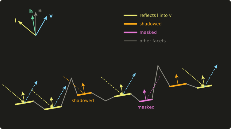
Microfacet theory (マイクロファセット理論) turns this picture into a BRDF with three ingredients:
- the normal distribution function (NDF, 法線分布関数) : how many facets face ,
- the masking–shadowing function (マスキング・シャドウイング関数, the geometry term) : which fraction of them is both lit and visible,
- the Fresnel term : how much one facet mirrors at its own angle of incidence (chapter 12, section 12.4).
The facets are assumed to be much larger than the wavelength of light (so geometric optics applies) and much smaller than a pixel (so we only care about their statistics).
The Cook–Torrance formula, derived
Robert Cook and Kenneth Torrance (1982) combined them into the formula of chapter 12:
Here's where the 4 and the two cosines come from.
First, what means exactly: for a piece of surface of area , the facets whose normals lie in a small solid angle around have a total area of .
Projected onto the macroscopic surface, every facet covers its area times , and all facets together cover exactly , which gives the normalization every NDF must satisfy:
Now follow the light step by step.
- Light of radiance arrives from a small solid angle around . The facets facing see it at the angle , so they receive the power .
- A fraction of it is mirrored, and a fraction of that is neither shadowed nor masked.
- The mirrored light leaves into a solid angle around . Tilting a mirror by an angle turns the reflected ray by twice that angle, so the reflected directions are spread four times wider (two in each of two dimensions) than the facet normals; the exact relation is .
- The outgoing radiance is power per projected area per solid angle .
Putting it together, with (that's what "half vector" means):
The BRDF is outgoing radiance per incoming irradiance , and dividing gives exactly the Cook–Torrance formula.
The formula is symmetric in and as long as is, so it's reciprocal for free.
D: Beckmann, GGX and Blinn–Phong
Write for the angle between and , and for the roughness parameter of the distribution (small = smooth).
Three distributions are worth knowing:
- The Beckmann distribution (ベックマン分布) comes from the optics of rough surfaces (Petr Beckmann and André Spizzichino, 1963), assuming Gaussian-distributed slopes. Cook and Torrance used it in 1982.
- GGX was introduced to graphics by Bruce Walter, Stephen Marschner, Hongsong Li and Kenneth Torrance in 2007 ("Microfacet Models for Refraction through Rough Surfaces"); the same function had been derived by T. S. Trowbridge and K. P. Reitz in 1975 for surfaces made of tiny ellipsoids, so it's also called the Trowbridge–Reitz distribution (トローブリッジ・ライツ分布). Today it's the default almost everywhere.
- Blinn–Phong as an NDF: chapter 10's with the factor is a valid normalized distribution, and makes it look like Beckmann with roughness (Walter et al. give this correspondence). This is the deep reason Blinn–Phong was a good model.
Checking the normalization of GGX takes three lines.
With , , and the substitution (so ):
The C++ program in section 22.4 confirms it numerically for three roughness values, and Beckmann and normalized Blinn–Phong pass the same test (I checked them in Python too).
Worked values. At both GGX and Beckmann have their peak ; for that's .
Away from the peak they differ:
| GGX, | Beckmann, | |
|---|---|---|
| 0° | 5.093 | 5.093 |
| 10° | 2.415 | 3.293 |
| 20° | 0.671 | 0.784 |
| 30° | 0.226 | 0.0437 |
| 45° | 0.0705 | 0.0000023 |
Let's do the 30° GGX value by hand: , so the bracket is , its square is , and .
Beckmann's Gaussian falls off a cliff; GGX keeps a long tail: at 45° it's about 30,000 times larger.
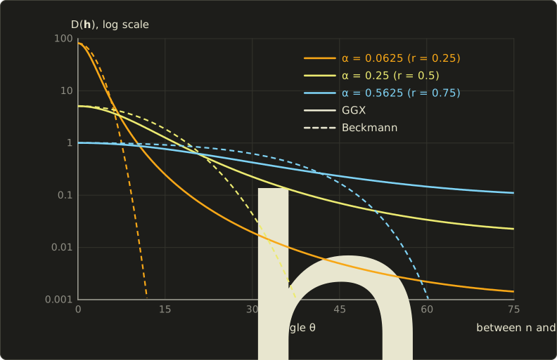
That tail is what you see on real materials: a sharp highlight surrounded by a soft glow (look at a chrome tap or a car's clear coat under a lamp).
Measured materials are often fit better by GGX, which is one reason it replaced Beckmann (Walter et al. showed this for several rough glass samples; the Disney measurements of Burley 2012, below, pointed the same way).
Even longer or shorter tails can be dialed in with "generalized" versions (GTR, Student's t), which I'll only name here.
The roughness remapping
The in the formulas is not what artists type in.
Brent Burley (Disney, "Physically-Based Shading at Disney", SIGGRAPH 2012) found that a slider for itself bunches all the interesting materials into its lower end, and that using a perceptual roughness (知覚的ラフネス) with
spreads the visible change evenly; Unreal Engine 4 (Karis 2013) and glTF 2.0 adopted the same remapping.
When someone says "roughness 0.5" they mean , :
| roughness | GGX peak | |
|---|---|---|
| 0.25 | 0.0625 | 81.49 |
| 0.5 | 0.25 | 5.093 |
| 0.75 | 0.5625 | 1.006 |
| 1 | 1 | 0.3183 |
At GGX becomes the constant : facet normals point in all directions equally often (in projected area).
At it collapses to a single direction: a perfect mirror, which a point light can never hit exactly, so real-time shaders clamp the roughness to a small minimum (the OpenGL series uses 0.03).
G: Smith masking and shadowing
Bruce Smith (1967), working on the scattering of radio waves by rough surfaces, computed the probability that a point on a random surface is visible from a direction.
His idea, adopted in graphics, is to assume the heights and slopes of the surface are uncorrelated from point to point, which turns masking into a single function of the direction, , determined by the NDF.
The fraction of facets visible from is then
Eric Heitz ("Understanding the Masking-Shadowing Function in Microfacet-Based BRDFs", JCGT 2014) sorted out the possible ways to combine masking (towards the eye) and shadowing (towards the light):
- Separable: , as if being lit and being visible were independent events.
- Height-correlated (高さ相関): . A facet low in a valley is likely to be both shadowed and masked, a facet on a peak likely to be neither; this form accounts for that and is more accurate. It's always a little larger than the separable one, because .
A useful test, again from Heitz: for any viewing direction, the visible projected facet area must equal the projected area of the macro-surface,
(the "weak white furnace test"); I checked numerically that GGX with this satisfies it to five digits for = 0.25, 0.5 and 1, at = 1 and 0.5.
Because needs a square root and a tangent, real-time code often uses Schlick's approximation with (or ).
With it matches Smith–GGX exactly at (both become ) and approximately elsewhere:
| Smith exact, | Schlick, | Smith exact, | |
|---|---|---|---|
| 0.8 | 0.9914 | 0.9697 | 0.8889 |
| 0.6 | 0.9737 | 0.9231 | 0.7500 |
| 0.2 | 0.7749 | 0.6667 | 0.3333 |
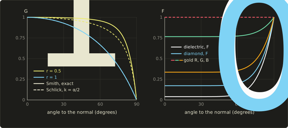
matters most at grazing angles and for rough surfaces, where it keeps the of the denominator from exploding.
A convenient trick: and the denominator are usually computed together as the visibility term ; for the height-correlated GGX form a little algebra (write with ) gives
which has no division by a cosine that could be zero.
That's the form the shader in section 22.4 uses.
Karis (Unreal Engine 4, 2013) used Schlick's form with for point lights (a deliberate remapping that makes rough surfaces less bright at grazing angles) and for image-based lighting; the OpenGL series follows him, so don't be surprised to see both.
F: Fresnel with the half vector
Each facet is a mirror, so it reflects the Fresnel fraction of chapter 12 for its own angle of incidence, which is the angle between (or ) and the facet normal , not :
, the reflectance at normal incidence, is the one material constant of the specular term:
| Material | (linear) | note |
|---|---|---|
| water | 0.02 | |
| glass, plastic, most dielectrics | 0.04 | |
| diamond | 0.17 | |
| gold | (1.0, 0.766, 0.336) | colored |
| copper | (0.955, 0.638, 0.538) | colored |
| silver, aluminum | about 0.91 to 0.99 in all channels | nearly white |
The dielectric values come from chapter 12's ; going backwards, , so the typical range 0.02 to 0.05 means between 1.33 and 1.58.
Metals reflect 50 to 100% head-on and their depends on the wavelength, which is their color.
Published tables differ by a few percent (gold's green channel is quoted between about 0.71 and 0.77, depending on the measurement); I use the values of the OpenGL series.
The lobe
Here is the specular BRDF (with ) for light at 45°, plotted as in each outgoing direction of the plane of incidence, the share of the reflected light that goes there:
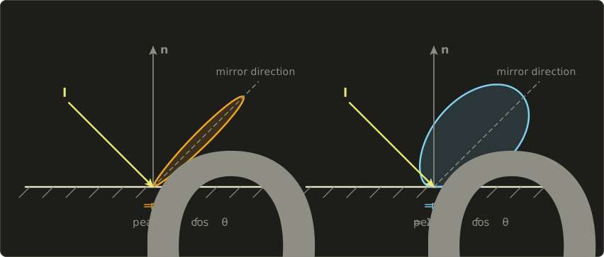
The rough lobe is 33 times lower at its peak but much wider, so the total is similar: that's normalization at work.
Its peak lies at 42°, slightly towards the normal, because the factor and masking eat the grazing side.
The BRDF value by itself behaves the other way: it grows towards grazing directions (the and Fresnel win), which is why rough surfaces show bright reflections at grazing angles, the "off-specular peaks" Torrance and Sparrow described for real materials in 1967.
Exam points
These tie back to the reflection models of chapter 10 and the BRDF of chapter 12:
- Microfacet BRDF: . D = how many facets face (normal distribution), G = how many are neither shadowed nor masked (geometric attenuation), F = Fresnel reflectance of one facet, evaluated with the angle between and .
- An NDF is normalized by (projected area), not by .
- A narrower highlight must be brighter: normalized lobes conserve energy, Phong's unnormalized one doesn't.
- Phong's specular term has no Fresnel effect and, as a BRDF, isn't reciprocal.
22.4 One light, fully worked
Let's evaluate everything at one point, with the geometry of chapter 10's worked example so you can compare:
- , , .
- A point light of radiant intensity W/sr at distance .
- Material: base color (orange), metallic , roughness . The metallic parameter and the rules for and the diffuse part are explained in section 22.5; for a dielectric they give and .
Step 1: the dot products.
Chapter 10 found with length , so .
So each facet that matters is hit at 45° ().
Step 2: D. , , and exactly:
(The Blinn–Phong NDF with the matching gives here, same peak 5.093, a slightly different shape.)
Step 3: G. and :
The separable form gives , almost the same; both angles are far from grazing.
Karis's gives , noticeably darker, as intended for point lights.
Step 4: F. :
Step 5: the specular BRDF.
The same in all three channels: the highlight of a dielectric is white.
Step 6: the diffuse BRDF. The light that wasn't reflected at the surface, , enters and comes back out diffusely:
Step 7: the outgoing radiance. The irradiance is W/m², so
The same point in gold. With and the base color becomes , the diffuse part vanishes, and
Notice that is fine: a BRDF is a density per steradian, and only its integral (the albedo) must stay below 1.
Compared with chapter 10's Phong result for the same geometry, the dielectric's highlight is much weaker relative to its diffuse color (0.064 against 0.244, about a quarter, where chapter 10's Phong gave 0.332 against 0.48, about two thirds), but at grazing angles Fresnel will make it grow, which Phong never did.
In C++
Here are the formulas as a small program, using Vec3, dot and normalize from the Linear Algebra series' linalg.hh.
It checks the normalization of numerically (a midpoint sum over rings of ) and reproduces the two results above:
#include <cmath>
#include <cstdio>
#include <initializer_list>
#include "linalg.hh"

constexpr float kPi = 3.14159265358979f;

Vec3 mul(Vec3 a, Vec3 b) { return {a.x * b.x, a.y * b.y, a.z * b.z}; }
Vec3 lerp(Vec3 a, Vec3 b, float t) { return a + t * (b - a); }

// D: GGX / Trowbridge-Reitz normal distribution, alpha = roughness^2
float distributionGgx(float nDotH, float alpha) {
  float a2 = alpha * alpha;
  float d = nDotH * nDotH * (a2 - 1.0f) + 1.0f;
  return a2 / (kPi * d * d);
}

// Smith's Lambda for GGX; c = cosine between the normal and l (or v)
float smithLambda(float c, float alpha) {
  float tan2 = (1.0f - c * c) / (c * c);
  return 0.5f * (-1.0f + std::sqrt(1.0f + alpha * alpha * tan2));
}

// G2: height-correlated masking-shadowing
float geometrySmith(float nDotL, float nDotV, float alpha) {
  return 1.0f / (1.0f + smithLambda(nDotL, alpha) + smithLambda(nDotV, alpha));
}

// F: Schlick's approximation with an RGB F0
Vec3 fresnelSchlick(float cosTheta, Vec3 f0) {
  float w = std::pow(1.0f - cosTheta, 5.0f);
  return f0 + w * (Vec3{1, 1, 1} - f0);
}

// The full BRDF (diffuse + specular) of the metallic-roughness model.
Vec3 brdf(Vec3 n, Vec3 l, Vec3 v, Vec3 base, float metallic, float roughness) {
  Vec3 h = normalize(l + v);
  float nl = dot(n, l), nv = dot(n, v), nh = dot(n, h), vh = dot(v, h);
  float alpha = roughness * roughness;
  Vec3 f0 = lerp({0.04f, 0.04f, 0.04f}, base, metallic);
  Vec3 F = fresnelSchlick(vh, f0);
  float dg = distributionGgx(nh, alpha) * geometrySmith(nl, nv, alpha) / (4.0f * nl * nv);
  Vec3 kd = (1.0f - metallic) * (Vec3{1, 1, 1} - F);
  return mul(kd, base) / kPi + dg * F;
}

int main() {
  // 1. The NDF is normalized: integral of D(h) cos(theta_h) over the hemisphere = 1
  for (float r : {0.25f, 0.5f, 1.0f}) {
    const int steps = 200000;
    const double dTheta = (kPi / 2) / steps;
    double sum = 0;
    for (int i = 0; i < steps; ++i) {
      double th = (i + 0.5) * dTheta; // midpoint of ring i
      double c = std::cos(th), s = std::sin(th);
      sum += distributionGgx(c, r * r) * c * s * 2 * kPi * dTheta; // ring: 2 pi sin(th) dTheta sr
    }
    printf("r = %.2f: integral of D cos = %.4f\n", r, sum);
  }
  // 2. One light: the vectors of chapter 10, I = 50 W/sr at distance 5
  Vec3 n{0, 1, 0}, l{0, 0.6f, 0.8f}, v{0, 0.8f, -0.6f};
  float irradiance = 50.0f / 25.0f * dot(n, l);
  Vec3 orange = brdf(n, l, v, {0.8f, 0.4f, 0.2f}, 0.0f, 0.5f);
  Vec3 gold = brdf(n, l, v, {1.0f, 0.766f, 0.336f}, 1.0f, 0.5f);
  for (Vec3 f : {orange, gold}) {
    Vec3 radiance = irradiance * f;
    printf("f = (%.4f, %.4f, %.4f)  L = (%.4f, %.4f, %.4f)\n", f.x, f.y, f.z,
           radiance.x, radiance.y, radiance.z);
  }
  return 0;
}
r = 0.25: integral of D cos = 1.0000
r = 0.50: integral of D cos = 1.0000
r = 1.00: integral of D cos = 1.0000
f = (0.3077, 0.1857, 0.1247)  L = (0.3692, 0.2229, 0.1497)
f = (1.5154, 1.1615, 0.5113)  L = (1.8185, 1.3939, 0.6136)
In a shader
In a shader the same thing is usually written with the visibility term of section 22.3, and the light is given as the irradiance it delivers to a surface facing it (, for a point light ):
static const float PI = 3.14159265;

float distributionGgx(float nDotH, float alpha) {
  float a2 = alpha * alpha;
  float d = nDotH * nDotH * (a2 - 1.0) + 1.0;
  return a2 / (PI * d * d);
}

// V = G2 / (4 (n.l)(n.v)) for height-correlated Smith-GGX
float visibilitySmithGgx(float nDotL, float nDotV, float alpha) {
  float a2 = alpha * alpha;
  float lv = nDotL * sqrt(nDotV * nDotV * (1.0 - a2) + a2);
  float vl = nDotV * sqrt(nDotL * nDotL * (1.0 - a2) + a2);
  return 0.5 / (lv + vl);
}

float3 fresnelSchlick(float cosTheta, float3 f0) {
  return f0 + (1.0 - f0) * pow(1.0 - cosTheta, 5.0);
}

// Outgoing radiance for one light that delivers lightIrradiance to a surface facing it.
float3 shadePbr(float3 n, float3 v, float3 l, float3 lightIrradiance,
                float3 baseColor, float metallic, float roughness) {
  float3 h = normalize(l + v);
  float nDotL = saturate(dot(n, l));
  float nDotV = max(dot(n, v), 1e-4);
  float nDotH = saturate(dot(n, h));
  float vDotH = saturate(dot(v, h));
  float alpha = max(roughness, 0.03) * max(roughness, 0.03);
  float3 f0 = lerp(float3(0.04, 0.04, 0.04), baseColor, metallic);
  float3 F = fresnelSchlick(vDotH, f0);
  float3 specular = distributionGgx(nDotH, alpha) * visibilitySmithGgx(nDotL, nDotV, alpha) * F;
  float3 diffuse = (1.0 - F) * (1.0 - metallic) * baseColor / PI;
  return (diffuse + specular) * lightIrradiance * nDotL;
}
const float PI = 3.14159265;
float distributionGgx(float nDotH, float alpha) {
float a2 = alpha * alpha;
float d = nDotH * nDotH * (a2 - 1.0) + 1.0;
return a2 / (PI * d * d);
}
// V = G2 / (4 (n.l)(n.v)) for height-correlated Smith-GGX
float visibilitySmithGgx(float nDotL, float nDotV, float alpha) {
float a2 = alpha * alpha;
float lv = nDotL * sqrt(nDotV * nDotV * (1.0 - a2) + a2);
float vl = nDotV * sqrt(nDotL * nDotL * (1.0 - a2) + a2);
return 0.5 / (lv + vl);
}
vec3 fresnelSchlick(float cosTheta, vec3 f0) {
return f0 + (1.0 - f0) * pow(1.0 - cosTheta, 5.0);
}
// Outgoing radiance for one light that delivers lightIrradiance to a surface facing it.
vec3 shadePbr(vec3 n, vec3 v, vec3 l, vec3 lightIrradiance,
vec3 baseColor, float metallic, float roughness) {
vec3 h = normalize(l + v);
float nDotL = clamp(dot(n, l), 0.0, 1.0);
float nDotV = max(dot(n, v), 1e-4);
float nDotH = clamp(dot(n, h), 0.0, 1.0);
float vDotH = clamp(dot(v, h), 0.0, 1.0);
float alpha = max(roughness, 0.03) * max(roughness, 0.03);
vec3 f0 = mix(vec3(0.04), baseColor, metallic);
vec3 F = fresnelSchlick(vDotH, f0);
vec3 specular = distributionGgx(nDotH, alpha) * visibilitySmithGgx(nDotL, nDotV, alpha) * F;
vec3 diffuse = (1.0 - F) * (1.0 - metallic) * baseColor / PI;
return (diffuse + specular) * lightIrradiance * nDotL;
}static const float PI = 3.14159265;
float distributionGgx(float nDotH, float alpha) {
float a2 = alpha * alpha;
float d = nDotH * nDotH * (a2 - 1.0) + 1.0;
return a2 / (PI * d * d);
}
// V = G2 / (4 (n.l)(n.v)) for height-correlated Smith-GGX
float visibilitySmithGgx(float nDotL, float nDotV, float alpha) {
float a2 = alpha * alpha;
float lv = nDotL * sqrt(nDotV * nDotV * (1.0 - a2) + a2);
float vl = nDotV * sqrt(nDotL * nDotL * (1.0 - a2) + a2);
return 0.5 / (lv + vl);
}
float3 fresnelSchlick(float cosTheta, float3 f0) {
return f0 + (1.0 - f0) * pow(1.0 - cosTheta, 5.0);
}
// Outgoing radiance for one light that delivers lightIrradiance to a surface facing it.
float3 shadePbr(float3 n, float3 v, float3 l, float3 lightIrradiance,
float3 baseColor, float metallic, float roughness) {
float3 h = normalize(l + v);
float nDotL = saturate(dot(n, l));
float nDotV = max(dot(n, v), 1e-4);
float nDotH = saturate(dot(n, h));
float vDotH = saturate(dot(v, h));
float alpha = max(roughness, 0.03) * max(roughness, 0.03);
float3 f0 = lerp(float3(0.04, 0.04, 0.04), baseColor, metallic);
float3 F = fresnelSchlick(vDotH, f0);
float3 specular = distributionGgx(nDotH, alpha) * visibilitySmithGgx(nDotL, nDotV, alpha) * F;
float3 diffuse = (1.0 - F) * (1.0 - metallic) * baseColor / PI;
return (diffuse + specular) * lightIrradiance * nDotL;
}A quick check that really is , with the numbers of the worked example (, , , so ):
The OpenGL series implements a variant of this function (with Schlick's ) in its chapter 24, together with normal maps from its chapter 22.
22.5 The metallic–roughness workflow
Two kinds of matter
What happens to the light a facet doesn't mirror (the ) splits all materials into two classes:
- Dielectrics (誘電体, non-metals: plastic, wood, stone, paint, skin, water) mirror only a few percent, uncolored (). The rest enters, is scattered by pigments, and comes back out in all directions, colored by what wasn't absorbed: the diffuse reflection, whose color we call the albedo.
- Metals (金属, conductors) mirror 50 to 100%, with a colored . What enters is absorbed within nanometers by the free electrons, so a metal has no diffuse reflection at all.
So in principle a material needs two colors: a diffuse color and an .
But for real materials they're never both "free": dielectrics have a nearly fixed gray , metals have no diffuse color.
The parameters
The metallic–roughness workflow (メタリック・ラフネスワークフロー), popularized by Burley's Disney model (2012) and Unreal Engine 4 (2013) and standardized by glTF 2.0, exploits that with three main parameters:
- base color (ベースカラー) : the albedo for a dielectric, for a metal,
- metallic (メタリック, 金属度) from 0 to 1,
- roughness (ラフネス, 粗さ) from 0 to 1, with .
From these:
and the BRDF is the one of section 22.4,
The glTF specification (Appendix B) writes the same thing as a blend: a dielectric BRDF mix(diffuse, specular, F) with , a metal BRDF whose Fresnel uses the base color as , and mix(dielectric, metal, metallic) between them; multiplying out gives the formula above.
Its reference implementation uses GGX for and writes the visibility term as a product of a light factor and a view factor (the separable Smith–GGX form), and it explicitly allows implementations to vary.
Worked example with :
| metallic | diffuse color | what it is | |
|---|---|---|---|
| 0 | (0.04, 0.04, 0.04) | (0.8, 0.4, 0.2) | orange plastic: orange body, white highlight |
| 1 | (0.8, 0.4, 0.2) | (0, 0, 0) | an (imaginary) orange metal: orange reflections, nothing else |
| 0.5 | (0.42, 0.22, 0.12) | (0.4, 0.2, 0.1) | no real material |
Intermediate metallic values don't describe any real matter; they exist for the transitions in textures (a pixel half on rust, half on bare steel, or the filtered texel at the border between them).
Most texels of a well-made metallic map are exactly 0 or 1.
Here is the whole space, rendered with exactly the formulas of this chapter (one directional light plus a sky, with the image-based lighting of section 22.6), for a base color of gold:
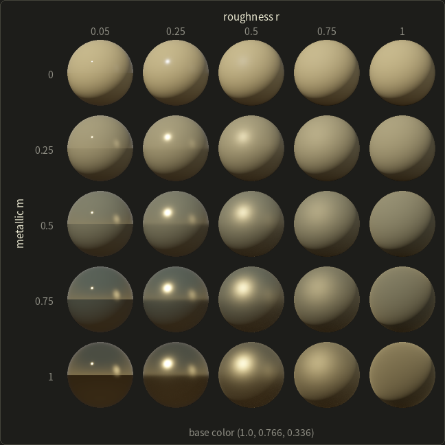
Things to look for: along the top row the highlight is white and the sphere's color comes from the diffuse term; the smooth plastic sphere shows the horizon only at its rim, where Fresnel rises.
Along the bottom row the reflections themselves are golden and there's no diffuse shading at all; the rough gold sphere still looks metallic because its "diffuse-looking" glow is really a very blurry, golden reflection.
Down a column, the diffuse light fades and the reflections take over.
Textures
In glTF the parameters come from factors times textures:
baseColorTexturestores color, encoded as sRGB; the GPU decodes it to linear before shading (chapter 3, section 3.7).metallicRoughnessTexturestores roughness in the green channel and metallic in the blue channel, as linear data. Roughness and metallic aren't colors; decoding them as sRGB would bend the values.normalTexture(chapter 11's normal maps),occlusionTexture(baked ambient occlusion, red channel, which glTF applies to indirect light only) andemissiveTexturecomplete the set.
These are the "roughness and metallic maps" chapter 11 (section 11.10) mentioned: a scratch in a roughness map makes the highlight sharper or blurrier exactly there, a painted logo on bare metal is a 0 in the metallic map.
Real-world albedos also give useful limits for base colors of dielectrics: hardly anything is darker than about 0.03 (charcoal) or brighter than about 0.9 (fresh snow), so a base color of pure black or pure white is a warning sign.
The specular–glossiness workflow
The older specular–glossiness workflow (スペキュラー・グロッシネスワークフロー) stores the two colors separately: a diffuse color, a specular color ( as RGB), and a glossiness , usually .
Converting from metallic–roughness is direct:
Gold (, , ) becomes diffuse (0, 0, 0), specular (1.0, 0.766, 0.336) and glossiness 0.7.
The other direction isn't always possible: diffuse (0.5, 0.5, 0.5) with specular (0.2, 0.2, 0.2) is neither a 4% dielectric nor a black-diffuse metal.
That freedom is both the advantage (gemstones, , and other unusual dielectrics) and the danger (diffuse 0.9 plus specular 0.9 creates energy) of the specular workflow; it also needs an RGB specular texture where metallic–roughness needs one channel.
glTF's extension for it, KHR_materials_pbrSpecularGlossiness, was archived by Khronos in 2021 (still readable, no longer recommended for new files); the extensions KHR_materials_ior and KHR_materials_specular now give metallic–roughness materials control over the dielectric instead.
Why this beats chapter 10's model
Compare with the Phong parameters of chapter 10:
- Energy: couples diffuse and specular, and the normalized couples the highlight's width and height. An artist can't make a material that glows in the dark.
- Fresnel is built in, so every material gets brighter reflections at grazing angles, the main thing that made chapter 10's renders look like plastic.
- Few, meaningful parameters: roughness means the same thing in the sun, in a cave and in an environment reflection, so materials can be shared between scenes, tools and engines (that's what glTF is for).
- Ambient light disappears as a separate concept: the environment is lit through the same BRDF (next section).
22.6 Image-based lighting with PBR
Chapter 12 (section 12.13) introduced image-based lighting with HDR environment maps and showed that a white Lambertian ball in a uniform sky shows exactly the sky's radiance.
For a real environment and our full BRDF, each pixel would have to evaluate
over the whole hemisphere, every frame.
Real-time renderers precompute as much of it as possible, separately for the two terms.
Diffuse: irradiance and spherical harmonics
The diffuse term is a constant times the irradiance:
depends only on the normal, so it can be stored as an irradiance map (放射照度マップ), a small cube map indexed by .
Even smaller: the integral against the clamped cosine is a strong blur that removes all fine detail, so a handful of numbers suffice.
Ravi Ramamoorthi and Pat Hanrahan ("An Efficient Representation for Irradiance Environment Maps", SIGGRAPH 2001) showed that 9 spherical harmonics (球面調和関数, SH) coefficients per color channel are enough: SH are to functions on the sphere what sine waves are to a 1D signal, grouped into bands of increasing frequency ( functions per band; bands 0 to 2 make ).
The clamped-cosine blur simply multiplies band by a constant :
| band | 0 | 1 | 2 | 3 | 4 |
|---|---|---|---|---|---|
| 0 |
Band 3 vanishes exactly and band 4 is only 4% of band 0, so dropping everything above band 2 costs very little.
(The projection itself, and SH light probes in games, are worked through in chapter 24.)
Worked example with just bands 0 and 1.
Take a sky whose radiance depends only on how far up a direction points: with and (0.8 at the zenith, 0.5 at the horizon, 0.2 straight down).
The constant is pure band 0 and the linear pure band 1, so the irradiance is
| normal | white plaster, : | |
|---|---|---|
| up | 2.1991 | 0.560 |
| sideways | 1.5708 | 0.400 |
| down | 0.9425 | 0.240 |
I checked these three values by integrating the sky over the sphere numerically; they agree to five digits.
The sphere grid of section 22.5 is lit exactly this way, with 9 coefficients projected from its sky.
Specular: the split-sum approximation
The specular term is harder: it depends on , the roughness and , far too many dimensions to tabulate.
Brian Karis ("Real Shading in Unreal Engine 4", SIGGRAPH 2013) proposed the split-sum approximation (スプリットサム近似): estimate the integral with samples (Monte Carlo, chapter 23) and split the sum into two factors that can each be precomputed:
- The prefiltered environment map (プリフィルタ済み環境マップ) is the environment blurred with the shape of the GGX lobe. Its mip levels hold increasing roughness, and it's looked up in the reflection direction. To make it independent of , Karis assumes (looking at the surface head-on). That loses the long, stretched reflections you see at grazing angles on a wet street: that's the price of the method.
- The BRDF integral is the directional albedo of the specular lobe, against a white environment. It depends on , the roughness and . Writing Schlick as with pulls out: the integral becomes , and and depend only on and roughness. That's a small 2D texture, the BRDF lookup table (BRDF LUT).
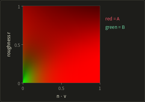
At run time the specular IBL is prefiltered(r, roughness) * (F0 * A + B): two texture lookups.
Checks you can do by hand. At roughness 0 every half vector is , so , , and the table must hold , : then is exactly Schlick's formula.
At : , , a perfect mirror of strength .
At (60°): , , and for glass , chapter 12's Schlick value at 60°.
With roughness the numbers drop; the table in the picture (computed with Schlick's and , as the OpenGL series does) has, for example, , at , , so glass there reflects of a white environment.
How the sums are computed efficiently (importance sampling of GGX) is part of chapter 23; the OpenGL series builds all three textures in its chapter 24.
Energy lost by single scattering
Run the white furnace test on the specular lobe alone: a metal with (a perfect mirror material) in a uniform white environment.
Its directional albedo is with , and it should be 1.
It isn't:
| roughness | 0.25 | 0.5 | 0.75 | 1 |
|---|---|---|---|---|
| albedo at | 0.996 | 0.916 | 0.627 | 0.307 |
For there's even a closed form: , , and at the albedo is .
Seventy percent of the light vanishes.
Where does it go?
The model counts light that is mirrored once; light that hits a facet, is mirrored into a neighboring facet and leaves after two or more bounces is simply dropped by .
On smooth surfaces that's negligible, on rough metals it makes them visibly too dark:
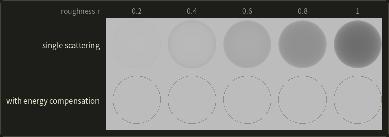
Christopher Kulla and Alejandro Conty Estevez (Sony Pictures Imageworks, SIGGRAPH 2017) added a second lobe that puts the missing energy back, and real-time engines use a cheap form of the same idea, a scale factor on the specular term (Emmanuel Turquin, 2019):
where is the albedo, which is from the LUT.
For the albedo becomes : the furnace test passes (bottom row).
For , the factor is for a perfect metal, but only for a dielectric, because a dielectric's facets lose most of the light to the surface on each bounce anyway.
22.7 More layers
The base model covers most opaque materials.
Real assets need a few more lobes; glTF defines them as extensions, Burley's Disney model has them as parameters, and engines implement similar sets.
- Clear coat (クリアコート): a thin transparent varnish on top of the base (car paint, lacquered wood, carbon fiber). A second specular lobe with a fixed dielectric and its own roughness; the base layer below is dimmed by the light the coat reflected, roughly . In glTF:
KHR_materials_clearcoat. - Sheen (シーン): velvet and other cloth with fibers standing up from the surface scatter light towards grazing angles, a soft bright rim. It uses an inverted-looking distribution (the "Charlie" sheen of Conty Estevez and Kulla, 2017, is one example). In glTF:
KHR_materials_sheen. - Anisotropy (異方性): brushed metal, hair and satin have highlights stretched in one direction. The GGX distribution gets two roughnesses, along the tangent and the bitangent (chapter 11's tangent space): , which reduces to ordinary GGX when (I checked its normalization numerically for ). In glTF:
KHR_materials_anisotropy. - Subsurface scattering and transmission: the BSSRDF of chapter 12 (section 12.6). Real-time engines approximate it with blurred diffuse lighting on skin, wrapped lighting or precomputed profiles; film renderers trace it. glTF has
KHR_materials_transmissionandKHR_materials_volumefor thin and thick transparent objects; volumes as such are chapter 28. - Rough diffuse: Lambert is ideal for smooth matte surfaces, but rough ones (clay, the moon) look flatter and brighter at grazing angles. Burley's diffuse term multiplies Lambert by with , where is the angle between and . For , light and eye together at 80° from the normal (, ) the factor is 2.49, a bright retro-reflection; for it's 0.65, a darkening at grazing angles. (It isn't exactly energy conserving; other rough-diffuse models, from Oren and Nayar's (1994) to recent energy-preserving ones, handle this differently.)
Burley's model, the Disney principled BRDF (ディズニーのプリンシプルドBRDF), put this philosophy into words: parameters should be intuitive, range from 0 to 1, and every combination should be plausible.
It has a base color and ten scalar parameters (subsurface, metallic, specular, specular tint, roughness, anisotropic, sheen, sheen tint, clear coat, clear coat gloss), and most production material models today descend from it.
22.8 Area lights in real time
Point and directional lights are mathematical idealizations.
Real lamps have a size, which gives soft shadows (chapter 11 and chapter 24) and highlights shaped like the lamp, a long streak from a fluorescent tube, a rectangle from a window.
Chapter 10 (section 10.9) promised the real-time approximations; here they are.
The exact answer is the rendering equation restricted to the light's solid angle :
Offline renderers sample it (chapter 23).
In real time there are two classic ideas.
Representative points
Replace the area light by one well-chosen point on it, the representative point (代表点), and shade with that point as an ordinary point light.
For the specular term, the best point is the one closest to the reflection ray: on a sphere light, the point where the reflection direction comes nearest to the sphere's center; on a tube light, the closest point on the segment.
Then the highlight takes the light's shape.
Because the lobe now "sees" a larger light, it must be widened and its energy renormalized; Karis (2013) does this by increasing according to the light's angular size.
It's cheap and convincing for spheres and tubes, less so for large rectangles.
Closed form for polygons, and linearly transformed cosines
For the diffuse term of a polygonal light there's an exact closed form, known since Lambert (1760): with the polygon's corners seen from the shaded point (as vectors from it), normalized to ,
(with , and the corners ordered counter-clockwise as seen from the point).
This number is the point-to-polygon form factor of chapter 12's radiosity, and the irradiance is times it.
Worked example. A square light with side 2 hangs at height 1 directly above the point, , corners :
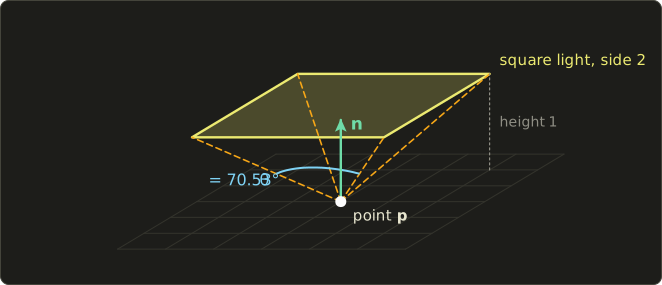
- Every corner is at distance . Two neighbors, e.g. and , have , so rad.
- Their cross product is proportional to (the plane through the point and that edge), so its unit vector is and the dot product with is 0.70711.
- By symmetry all four edges contribute the same: form factor .
With the irradiance is W/m², and a white plaster floor () shows .
(A brute-force numerical integration over the square gives the same 0.55413.)
Compare the "small light" approximation of section 22.1: W/m², more than twice too much, because most of the square is seen at a slant and from farther away than its center.
For the specular term, Eric Heitz, Jonathan Dupuy, Stephen Hill and David Neubelt ("Real-Time Polygonal-Light Shading with Linearly Transformed Cosines", SIGGRAPH 2016) found a beautiful trick.
Take the clamped cosine distribution, whose polygon integral we just computed in closed form, and apply a matrix to all its directions (a linear transformation, Linear Algebra chapter 8): stretching, skewing and scaling it produces lobes that can match the GGX lobe for a given view angle and roughness very closely.
These are linearly transformed cosines (LTC, 線型変換コサイン).
Integrating the transformed lobe over a polygon is the same as integrating the plain cosine over the polygon transformed by , and that's Lambert's formula again.
So at run time: look up for (, roughness) in a small precomputed table, transform the polygon's corners, clip to the horizon, apply the edge sum.
The result is accurate area lighting for rectangles and other polygons (the paper also handles textured lights, and later work extended the idea to lines and disks), and several engines use it at the time of writing.
The GLSL series, chapter 10 shows simpler area-light approximations in a shader.
22.9 Summary
- Radiance is measured per projected area; , the hemisphere is sr and . A Lambertian emitter has . Photometry weights the same quantities by : lumen, candela, lux, nit.
- A physical BRDF is positive, reciprocal and has directional albedo (white furnace test). Lambert () passes; Phong's specular term isn't reciprocal, and its albedo depends on the exponent unless normalized by .
- Microfacet BRDF: ; the 4 comes from . NDFs satisfy .
- GGX (Trowbridge–Reitz) has a long tail; Beckmann is Gaussian; normalized Blinn–Phong corresponds to . Perceptual roughness: .
- Smith: , height-correlated (Heitz 2014), Schlick's approximation with (or Karis's for point lights). Fresnel uses and (0.04 dielectrics, colored for metals).
- Metallic–roughness: , diffuse scaled by ; glTF stores roughness in G and metallic in B of a linear texture. Specular–glossiness stores diffuse and colors separately.
- IBL: diffuse from irradiance (, 9 SH coefficients, band factors , , ); specular from the split sum: prefiltered environment times from a BRDF LUT, assuming .
- Single-scattering microfacet models lose energy on rough surfaces ( albedo at head-on); energy compensation scales the lobe by .
- Extra lobes: clear coat, sheen, anisotropic GGX, subsurface/transmission, Burley's rough diffuse; the Disney principled BRDF.
- Area lights: representative points for spheres and tubes; Lambert's closed-form polygon integral for diffuse; linearly transformed cosines (Heitz et al. 2016) for GGX.
22.10 Key terms
| English | 日本語 |
|---|---|
| physically based rendering / shading (PBR) | 物理ベースレンダリング/シェーディング |
| radiometry / photometry | 放射測定/測光 |
| solid angle, steradian | 立体角、ステラジアン |
| projected area | 投影面積 |
| radiant flux / radiant intensity | 放射束/放射強度 |
| irradiance / radiant exitance | 放射照度/放射発散度 |
| radiance | 放射輝度 |
| luminous flux (lumen) / luminous intensity (candela) | 光束(ルーメン)/光度(カンデラ) |
| illuminance (lux) / luminance (cd/m², nit) | 照度(ルクス)/輝度(cd/m²、ニト) |
| BRDF | 双方向反射率分布関数 |
| reciprocity / energy conservation | 相反性/エネルギー保存 |
| directional albedo | 方向アルベド |
| white furnace test | ホワイトファーネステスト |
| normalization factor | 正規化係数 |
| microfacet theory | マイクロファセット理論 |
| half vector | ハーフベクトル |
| normal distribution function (NDF) | 法線分布関数 |
| GGX distribution (Trowbridge–Reitz) | GGX分布(トローブリッジ・ライツ分布) |
| Beckmann distribution | ベックマン分布 |
| masking–shadowing function | マスキング・シャドウイング関数(幾何減衰項) |
| height-correlated Smith G | 高さ相関のスミスのG |
| visibility term | 可視項 |
| Fresnel term, F0 | フレネル項、F0(垂直入射での反射率) |
| perceptual roughness | 知覚的ラフネス |
| dielectric / metal (conductor) | 誘電体(非金属)/金属(導体) |
| metallic–roughness workflow | メタリック・ラフネスワークフロー |
| base color / metallic / roughness | ベースカラー/メタリック(金属度)/ラフネス(粗さ) |
| specular–glossiness workflow | スペキュラー・グロッシネスワークフロー |
| irradiance map | 放射照度マップ |
| spherical harmonics (SH) | 球面調和関数 |
| prefiltered environment map | プリフィルタ済み環境マップ |
| split-sum approximation | スプリットサム近似 |
| BRDF lookup table (LUT) | BRDFルックアップテーブル(LUT) |
| multiple scattering / energy compensation | 多重散乱/エネルギー補償 |
| clear coat / sheen / anisotropy | クリアコート/シーン/異方性 |
| Disney principled BRDF | ディズニーのプリンシプルドBRDF |
| area light | 面光源 |
| representative point | 代表点 |
| form factor | 形態係数(フォームファクタ) |
| linearly transformed cosines (LTC) | 線型変換コサイン(LTC) |
22.11 Challenges
- ★ A Lambertian panel of 0.5 m² emits a total of 40 W. Compute its radiance. Then estimate the irradiance at a point 3 m away, with the panel facing the point and the point's surface tilted by 45°, using "radiance times solid angle times cosine". Convert a 1,200 lm isotropic bulb into candela and find the illuminance 1.5 m below it.
- ★ For roughness , compute , the GGX peak , and at and . Compute the Beckmann value at for the same and the ratio of the two.
- ★★ Show that , so normalized Blinn–Phong is a valid NDF. Then compute for GGX with at exactly and with Schlick's , and the separable and height-correlated for .
- ★★ A material has base color (0.9, 0.6, 0.3), metallic 0.25, roughness 0.4. Give its , diffuse color and the equivalent specular–glossiness parameters. Then compute the IOR that corresponds to , and the Schlick reflectance of that dielectric at .
- ★★★ A sky has radiance . Compute the irradiance for normals pointing up, sideways and down with the SH band factors, and explain why a normal pointing down still receives light. Then argue in words why the split-sum approximation can't produce the stretched reflections of street lights on a wet road, and why its BRDF table can be shared by every environment map.
Multiple choice
Q1 ★ Which of the following statements about the metallic–roughness workflow is correct?
| A | A metallic value of 0.5 describes a typical real material, such as most painted metals. |
| B | Roughness is stored in an sRGB texture, because it is shown to the artist as a color. |
| C | For a fully metallic material, the base color is used as F0 and the diffuse reflection is zero. |
| D | For a dielectric, the base color is used as F0, and the diffuse color is fixed at 0.04. |
| E | The roughness r is used directly as the alpha of the GGX distribution, without any remapping. |
Q2 ★ Which of the following statements about the terms of the microfacet (Cook–Torrance) BRDF is correct?
| A | The normal distribution function D is normalized so that its integral over the hemisphere, without any cosine, equals 1. |
| B | The Fresnel term F is evaluated with the angle between the macroscopic normal n and the light direction. |
| C | The factor 4 in the denominator corrects for the four color channels RGBA. |
| D | The GGX distribution falls off faster than the Beckmann distribution far from its peak. |
| E | The geometry term G accounts for microfacets that are hidden from the light or from the viewer by other microfacets. |
Q3 ★★ Which of the following statements about image-based lighting with the split-sum approximation is correct?
| A | The prefiltered environment map stores the irradiance for Lambertian diffuse reflection, one level per base color. |
| B | It reproduces the stretched reflections at grazing angles exactly, because it evaluates the full BRDF for every view direction. |
| C | The BRDF lookup table must be recomputed whenever the environment map changes. |
| D | The BRDF lookup table depends only on n · v and the roughness, not on the environment map, so it can be shared by all environments. |
| E | It needs no precomputation; the GGX lobe is integrated over the whole environment map for every pixel at run time. |
22.12 Practical assignment
Evaluate a physically based material by hand at three viewing angles, check the normal distribution numerically, and compare with chapter 10's Phong model.
You need a calculator (with , powers and trigonometric functions), paper, a ruler and a protractor; graph paper helps for the plot in step 7.
The setup is a 2D cross-section (everything happens in the plane ): the surface normal is , the light comes from on the left, , as a directional light that delivers W/m² to a surface facing it.
The material is blue plastic: base color , metallic 0, roughness .
- Draw the surface, and with the protractor, and three view directions on the right side at = 20°, 40° (the mirror direction) and 70°: .
- Half vectors. For each view, compute and draw it. Write down , , and . (In 2D the half vector's angle is simply the average of the two signed angles, so you can check with the protractor.)
- D. Compute and the GGX value for each view.
- G. Compute and and the height-correlated for each view; for comparison also the Schlick form with .
- F and the BRDF. Compute with , the specular term , the diffuse term , and the outgoing radiance in all three channels.
- Normalization. Check for your with a midpoint sum over nine rings: for add up with rad. Make a small table.
- Plot the specular radiance (one channel) against with your three points, and add the Phong value times (chapter 10's form, with and the exponent ) for comparison.
How to check yourself: every has length 1 and lies between and ; is largest for the mirror view (where and ); is between 0 and 1 and decreases as grows, and Schlick's version comes out somewhat lower; is between 0.04 and 1 and grows as grows; the specular part is the same in all three channels while the diffuse part is blue; and your ring sum lands within about 2% of 1 (nine rings are coarse: 18 rings bring it closer).
If the ring sum is far from 1, check that you multiplied by (projected area) and used radians for .
Finally, look at your plot: the physically based highlight doesn't simply fall off beyond the mirror direction the way Phong's does.
Explain from the formula which factors make the difference.
コメント(0)
まだコメントはありません。
ログインするとコメント出来ます。