10. Hidden Surface Removal and Shading
In chapter 6 we took triangles all the way to pixels: we transformed them, clipped them, culled the back faces and rasterized what was left.
Two questions stayed open.
When two triangles land on the same pixel, which one do we see?
And what color should that pixel be?
This chapter answers both.
The first question is hidden surface removal: finding which surfaces are hidden behind others.
The second is shading: computing how bright a surface looks from the lights that shine on it, the material it's made of and the direction we look from.
Together they turn a set of colored triangles into a picture that looks solid.
Every renderer does both, from the z-buffer and the per-pixel lighting of a game engine to the ray-traced film frame of chapter 12.
For the exam, this chapter covers two syllabus items of area 4 (rendering): hidden surface removal (隠面消去) and shading (シェーディング).
That means the classic visibility algorithms (depth sort, Z-buffer, scanline, ray casting, BSP trees, area subdivision), the light sources, the reflection models (ambient, diffuse, specular; Phong and Blinn–Phong) and the shading methods (flat, Gouraud, Phong), plus transparency.
Shadows and texture mapping are chapter 11, and physically based reflection (BRDFs), ray tracing and global illumination are chapter 12.
The math we need is the dot product and the reflection formula from Linear Algebra chapter 4, normalization from Linear Algebra chapter 3, and the edge functions and barycentric coordinates of chapter 6, section 6.9.
10.1 The visibility problem
Look at any scene: a cup on a table hides part of the table, the handle of the cup hides part of the cup, and the back of the cup is hidden by its own front.
In chapter 3 we met occlusion as one of the strongest depth cues: if something covers something else, it's in front.
A renderer that gets this wrong produces pictures that look like an X-ray, or worse, where far things are painted over near ones.
There are two versions of the problem:
- Hidden line removal (隠線消去): for wireframe drawings, remove the parts of the edges that are hidden by faces. This was the first problem solved, for CAD plots on pen plotters (Roberts in 1963 for convex objects, Appel's "quantitative invisibility" in 1967).
- Hidden surface removal (隠面消去), also called visible surface determination: for shaded pictures, decide for every pixel which surface is visible there.
Today almost everything is shaded, so the rest of the chapter is about surfaces; a hidden-line drawing can be made with any hidden-surface method too, by filling the faces with the background color and drawing their edges on top.
Object space and image space
The algorithms fall into two families:
- Object-space methods (物体空間法, also オブジェクト空間法) work with the geometry itself: they compare polygons with each other to find which is in front. The result is exact and independent of the resolution, but with polygons there are up to pairs to compare.
- Image-space methods (画像空間法) work per pixel: for each pixel, find the nearest surface. The answer is only as precise as the pixel grid, and the cost grows with (number of polygons) × (pixels each one covers), which in practice grows much more slowly than .
For a feeling of the numbers: 100,000 polygons give about pairs, while a 1920×1080 image has only about 2.07 million pixels.
Some methods mix the two: the painter's algorithm sorts in object space and lets the frame buffer do the rest.
Back-face culling is not enough
Section 6.4 introduced back-face culling (背面除去): drop every face whose normal points away from the eye, .
For a single convex closed object, like a cube or a sphere, that's already complete hidden surface removal: every front face is visible and every back face is hidden.
As soon as an object is concave (a cup, a character's arm in front of the body) or there are two objects, front faces can hide other front faces, and we need one of the methods below.
Back-face culling is still used with all of them as a cheap first step, since it removes about half of the faces of a closed mesh.
10.2 Depth sort and the painter's algorithm
The idea
A painter painting a landscape starts with the sky, then the mountains, then the trees, and finally the people in front, each layer covering what's behind it.
The painter's algorithm (画家のアルゴリズム) does the same: sort the polygons by depth, then draw them from the farthest to the nearest, simply overwriting the frame buffer.
The near polygons are drawn last, so they end up on top.
No depth memory is needed at all.
In its simplest form, each polygon is sorted by one number, for example its farthest vertex or its center.
That fails easily: a long floor polygon can have its farthest point behind a box standing on it, yet its near end is in front of the box.
The full depth sort method (奥行きソート法, Newell, Newell and Sancha, 1972) therefore sorts first by the farthest depth, and then checks every pair whose depth ranges overlap.
Polygon P (currently drawn before Q) may stay before Q if any of these tests succeeds, from cheapest to most expensive:
- The x extents of P and Q on the screen don't overlap.
- The y extents don't overlap.
- P lies entirely on the far side of Q's plane (seen from the eye).
- Q lies entirely on the near side of P's plane.
- The projections of P and Q on the screen don't overlap.
If all five fail, P might hide part of Q, so the algorithm swaps them and tests again.
Worked example: the plane test
Tests 3 and 4 use the plane equation of a polygon.
In camera space (eye at the origin, looking down −z), take polygon Q with the vertices , and .
All three satisfy , so Q lies in the plane
and is positive on one side and negative on the other.
The eye gives , so positive means "on the eye's side".
Now polygon P has the vertices , and :
All three are positive: P lies entirely on the eye's side of Q's plane, so Q can never hide P, and the safe order is Q first, then P.
Note that the depth ranges overlap (Q spans z from −8 to −4, P from −6 to −5), so sorting by one number alone could not have decided this safely.
Where it breaks: cycles and interpenetration
Two configurations defeat any ordering of whole polygons:
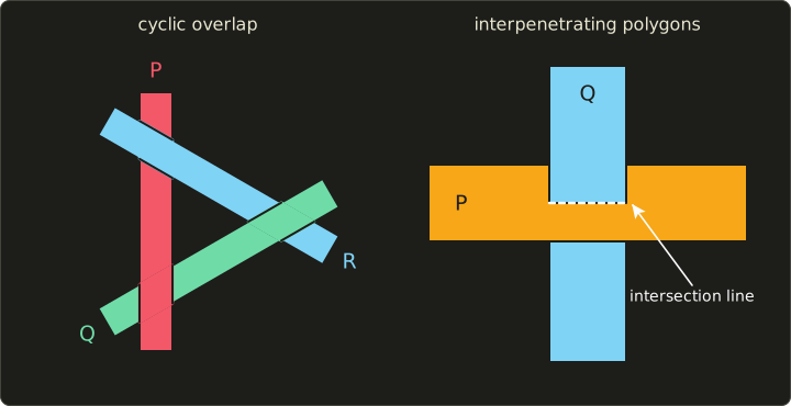
- Cyclic overlap (循環する重なり): P is on top of Q, Q on top of R, and R on top of P. Whichever bar you draw last covers both others completely, which is wrong.
- Interpenetration (貫通): Q passes through P. Above the intersection line Q is in front, below it P is in front. Neither "P first" nor "Q first" is correct.
The depth sort method detects these cases (a polygon that would be swapped a second time is part of a cycle) and splits one polygon along the other's plane, so that each piece can be ordered.
That works, but the number of polygons can grow, and the tests cost time.
In practice
The painter's algorithm is alive and well where sorting is cheap or unavoidable:
- 2D games, UI toolkits, SVG and PDF draw in a fixed layer order, which is exactly back-to-front painting.
- 3D engines draw semi-transparent objects sorted from back to front (section 10.12), because the Z-buffer can't handle them.
10.3 The Z-buffer method
The idea
The Z-buffer method (Zバッファ法) gives up on sorting altogether and decides visibility separately for every pixel.
Next to the color buffer it keeps a second image of the same size, the depth buffer or Z-buffer (深度バッファ, Zバッファ), which stores for each pixel the depth of the nearest surface drawn there so far.
The idea is usually credited to Ed Catmull (1974); Wolfgang Straßer described the same idea in his doctoral thesis the same year.
The algorithm:
- Clear the color buffer to the background color and the depth buffer to the farthest depth (1.0 for a depth range from 0 to 1).
- For every polygon, in any order, rasterize it. For every pixel it covers, compute the depth of the polygon at that pixel.
- Depth test (深度テスト): if is smaller (nearer) than the stored depth, write the polygon's color to the color buffer and to the depth buffer. Otherwise do nothing.
When all polygons are drawn, every pixel holds the color of the nearest surface.
This is the depth test of the GPU pipeline in section 6.5; OpenGL's default comparison, GL_LESS, is exactly "smaller is nearer".
How the depth is computed
The depth at a pixel comes from the vertex depths by the barycentric interpolation of section 6.9: .
The depth after the perspective division is an affine function of the screen position (that's why it may be interpolated linearly on the screen, as section 6.9 noted), so over a triangle it is a plane:
That makes it cheap: one pixel to the right adds the constant , one row up adds .
Worked example: two triangles that pass through each other
Here is a 10×8 pixel screen with two triangles (pixel centers at , y up, as in chapter 6):
- Red: vertices , , with depths 0.1, 0.9 and 0.26. Its depth plane is : it tilts away from us to the right.
- Blue: vertices , , with depths 0.3, 0.94 and 0.78. Its depth plane is : it tilts away from us upwards.
You can check the planes at the vertices: and .
The two planes are equal where , that is on the line : left of it red is nearer, right of it blue.
Let's draw red first, then blue, and follow two pixels.
Pixel (6, 2), center (6.5, 2.5).
After clearing, its depth is 1.
Red covers it with ; , so the pixel becomes red with depth 0.62.
Blue covers it with ; , so it becomes blue with depth 0.5.
Pixel (3, 5), center (3.5, 5.5).
Red: , so it becomes red with depth 0.38.
Blue: , which is not less than 0.38, so the depth test fails and the pixel stays red.
Now draw them the other way round, blue first.
Pixel (6, 2): blue writes 0.5, then red's 0.62 fails the test: blue.
Pixel (3, 5): blue writes 0.74, then red's 0.38 passes: red.
Same result.
Here is the whole screen with the final depth buffer values:
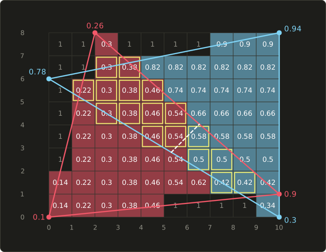
The yellow frames are the pixels where both triangles compete.
The boundary between red and blue inside that region follows the dashed line , as a staircase: the Z-buffer resolved the interpenetration that defeated the painter's algorithm, one pixel at a time, without any splitting.
Here's the same thing in C++, with the edge functions of section 6.9 and the linalg.hh header from the Linear Algebra series.
It draws the scene in both orders and prints the frame buffer:
#include <cstdio>
#include "linalg.hh"

struct Vertex {
  Vec2 p;  // screen position in pixels (y up)
  float z; // depth: 0 = near plane, 1 = far plane
};

const int W = 10, H = 8;
float depthBuf[H][W]; // the z-buffer
char colorBuf[H][W];  // the frame buffer (one letter per pixel)

float edgeFunction(Vec2 a, Vec2 b, Vec2 p) {
  return (b.x - a.x) * (p.y - a.y) - (b.y - a.y) * (p.x - a.x);
}

void clear() {
  for (int y = 0; y < H; ++y) {
    for (int x = 0; x < W; ++x) {
      depthBuf[y][x] = 1.0f; // as far away as possible
      colorBuf[y][x] = '.';  // background
    }
  }
}

// a, b, c counter-clockwise. (The top-left rule of chapter 6 is left out to keep it
// short; it only matters for edges that two triangles share.)
void drawTriangle(Vertex a, Vertex b, Vertex c, char name) {
  float area2 = edgeFunction(a.p, b.p, c.p);
  for (int y = 0; y < H; ++y) {
    for (int x = 0; x < W; ++x) {
      Vec2 p{x + 0.5f, y + 0.5f};
      float la = edgeFunction(b.p, c.p, p) / area2;
      float lb = edgeFunction(c.p, a.p, p) / area2;
      float lc = edgeFunction(a.p, b.p, p) / area2;
      if (la < 0 || lb < 0 || lc < 0) continue; // outside the triangle
      float z = la * a.z + lb * b.z + lc * c.z;  // interpolated depth
      if (z < depthBuf[y][x]) {                  // the depth test
        depthBuf[y][x] = z;
        colorBuf[y][x] = name;
      }
    }
  }
}

void print() {
  for (int y = H - 1; y >= 0; --y) { // top row first
    printf("%.*s\n", W, colorBuf[y]);
  }
}

int main() {
  Vertex r0{{0, 0}, 0.1f}, r1{{10, 1}, 0.9f}, r2{{2, 8}, 0.26f};
  Vertex b0{{10, 0}, 0.3f}, b1{{10, 8}, 0.94f}, b2{{0, 6}, 0.78f};

  clear();
  drawTriangle(r0, r1, r2, 'R');
  drawTriangle(b0, b1, b2, 'B');
  print();
  printf("pixel (6, 2): %c, depth %.2f\n\n", colorBuf[2][6], depthBuf[2][6]);

  clear();
  drawTriangle(b0, b1, b2, 'B'); // the other order
  drawTriangle(r0, r1, r2, 'R');
  print();
  printf("pixel (6, 2): %c, depth %.2f\n", colorBuf[2][6], depthBuf[2][6]);
  return 0;
}
..R....BBB
..RRBBBBBB
.RRRRBBBBB
.RRRRRBBBB
.RRRRRBBBB
.RRRRRBBBB
RRRRRRRBBB
RRRRR....B
pixel (6, 2): B, depth 0.50

..R....BBB
..RRBBBBBB
.RRRRBBBBB
.RRRRRBBBB
.RRRRRBBBB
.RRRRRBBBB
RRRRRRRBBB
RRRRR....B
pixel (6, 2): B, depth 0.50
Memory
The depth buffer needs one value per pixel, regardless of how many polygons the scene has.
At 1920×1080 with 24 bits (3 bytes) per pixel that's bytes, about 5.9 MiB; with 32 bits (a 32-bit float, or 24-bit depth plus 8-bit stencil as in chapter 6) it's 8,294,400 bytes, about 7.9 MiB.
When the Z-buffer was invented, that much memory was a serious cost; today it's nothing.
Precision and z-fighting
Chapter 5 showed that the depth stored after a perspective projection is not linear in the distance.
With the near plane , the far plane and the distance in front of the camera, the value in a 0 to 1 depth buffer is
(it's with the OpenGL of chapter 5, and Vulkan's projection gives the same value).
Its slope is , so one step of the stored value corresponds to a distance step of about
which grows with the square of the distance.
With a 24-bit integer depth buffer, .
For and (meters):
| Distance | with | with |
|---|---|---|
| 10 m | 0.06 mm | 0.006 mm |
| 100 m | 6.0 mm | 0.60 mm |
| 1000 m | 0.60 m | 6.0 cm |
At 100 m: m.
Two surfaces closer together than get the same stored depth, and which one wins the test changes from pixel to pixel and frame to frame: they flicker through each other.
That's z-fighting (Zファイティング), typically seen with a decal or a road marking lying on a road far away.
The second column shows the cheapest fix: moving the near plane from 0.1 to 1 makes every step ten times finer.
Other fixes (a 32-bit float buffer with "reversed Z", or a small depth offset for decals) are covered in Part 2.
Strengths and weaknesses
Strengths:
- Any order. No sorting at all; polygons can be streamed through in whatever order the program sends them.
- Any shape. Interpenetrating and cyclically overlapping polygons are handled per pixel, as are curved surfaces or anything else that can be rasterized with a depth per pixel.
- Simple and constant memory, which is why it's built into every GPU.
Weaknesses:
- Transparency. The buffer stores one surface per pixel. A semi-transparent surface needs to be mixed with what's behind it, and if the thing behind is drawn later, it fails the depth test and is lost (section 10.12).
- Aliasing. Visibility is decided at one point per pixel, so edges and intersection lines are jagged, like the staircase in the picture. MSAA stores a depth per sample to fix this (chapter 6 and Part 2).
- Precision, as computed above.
- Overdraw. A pixel may be shaded many times before the nearest surface arrives. GPUs reduce this with early-Z (the depth test before the fragment shader, chapter 6), and engines often draw the scene roughly front to back, or render depth alone first (a "depth pre-pass") and then shade only the visible fragments.
You'll configure the depth test yourself in the OpenGL series, chapter 15.
10.4 The scanline method
The scanline method (スキャンライン法) for hidden surfaces extends the polygon filling of section 6.8 to many polygons at once.
It was developed in the late 1960s and around 1970 (Wylie, Romney, Evans and Erdahl; Bouknight; Watkins), when memory for a whole Z-buffer was far too expensive.
It works one row (scanline) at a time:
- Keep the edge table and active edge list of chapter 6 for all polygons together, plus a polygon table with each polygon's plane equation and color, and an active polygon list with the polygons that cross the current scanline.
- On each scanline, sort the edge crossings by x. Between two neighboring crossings, the set of polygons present doesn't change. That piece of the scanline is a span (スパン).
- For each span, find the visible polygon: if only one polygon is present, it's that one; if several are, compare their depths. If one polygon is nearer at both ends of the span, it's nearer on the whole span (depths are linear along the scanline). If the order flips, the polygons intersect inside the span, so split it at the crossing point.
- Fill each span with its visible polygon.
Because the depth comparison happens once per span, not per pixel, and because the active lists change only a little from one scanline to the next (scanline coherence), the method is fast, and it needs depth memory for at most one scanline.
Worked example
Let's run the scanline (pixel row 3) through the two triangles of section 10.3.
The crossings of the edges with the scanline:
- Red's left edge from to : .
- Red's right edge from to : .
- Blue's lower edge from to : .
- Blue's right edge .
Sorted: 0.875, 4.167, 7.143, 10, giving three spans:
- : only red. Red.
- : both. Red's depth along the scanline is , blue's is the constant . At the left end red has 0.433, nearer than 0.58; at the right end red has 0.671, farther. The order flips, so we split where , at : red on , blue on .
- : only blue. Blue.
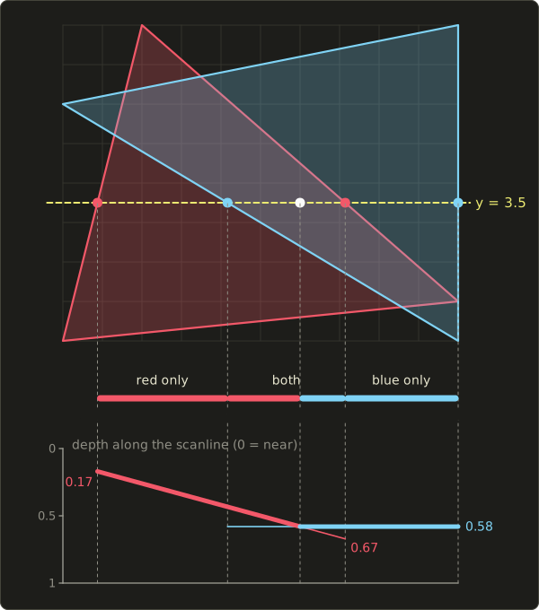
The pixel centers 1.5 to 5.5 lie in red spans and 6.5 to 9.5 in blue ones, which is row 3 of the Z-buffer result, .RRRRRBBBB.
Same picture, but on this row the depths were compared only at the two ends of the one span where both triangles are present, instead of once per covered pixel per triangle.
In practice
The scanline method was the standard in early hardware and in offline renderers when memory was precious, and its ideas (spans, coherence, incremental updates) live on in every rasterizer.
Its weakness is complexity: the bookkeeping of edges and polygons is much harder to build into parallel hardware than the Z-buffer's simple per-pixel test.
10.5 Ray casting
Ray casting (レイキャスティング法) turns the question around: instead of projecting polygons onto pixels, it starts at each pixel and asks what the eye sees through it.
For every pixel, it sends a ray (a half-line) from the eye through the pixel's position on the image plane, intersects the ray with every object, and takes the nearest intersection in front of the eye.
Arthur Appel described this in 1968.
A ray is with origin (the eye), direction and .
For a plane with normal and the equation , substituting the ray gives the hit parameter
(if the ray is parallel to the plane and misses it).
For a polygon, we then check whether the hit point lies inside the polygon, for example with the edge functions or barycentric coordinates of chapter 6.
Worked example
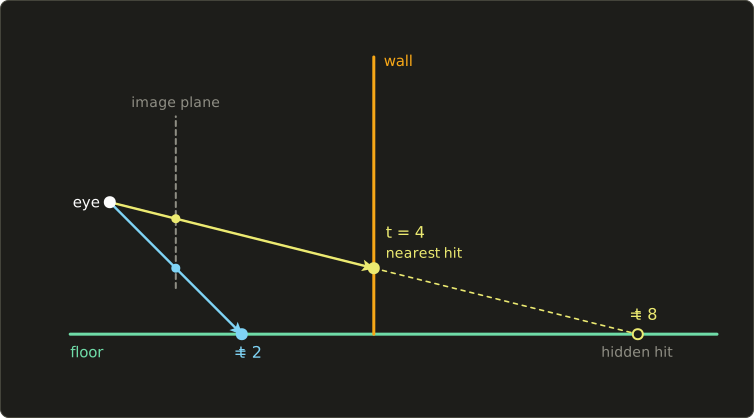
The eye is at the origin and looks down −z.
The scene has a floor, the plane , and a wall, the plane , which reaches from the floor up to .
The ray through one pixel has the direction (the pixel sits on the image plane at distance 1, slightly below the center).
- Wall: , . , hit point . Its height −1 lies between −2 and 2.2, so it's on the wall.
- Floor: , . , hit point , on the floor behind the wall.
The nearest hit is : this pixel shows the wall.
A second ray with hits the floor at , the point ; it would hit the plane of the wall at with the height −4, which is below the floor, outside the wall: a miss.
That pixel shows the floor.
In practice
Ray casting is an image-space method that needs no sorting, handles any surface that can be intersected with a ray (spheres, implicit surfaces, volumes, not just polygons) and has no depth buffer.
Its cost is the problem: naively every ray is tested against every object, so a 1920×1080 image of a scene with a million triangles needs about tests.
Acceleration structures (bounding volume hierarchies, grids, kd-trees) bring that down to roughly logarithmic cost per ray; they're explained in chapter 12.
Ray casting is also the first step of ray tracing, which continues the rays recursively for shadows, reflections and refraction (chapter 12), and it's how "picking" works in 3D editors: the ray under the mouse cursor tells you which object was clicked.
10.6 BSP trees
The idea
The painter's algorithm needs a back-to-front order, and sorting it every frame is expensive and sometimes impossible.
A BSP tree (binary space partitioning tree, BSP木 or BSP法; Fuchs, Kedem and Naylor, 1980) stores the scene so that a correct back-to-front order can be read off for any eye position, with no sorting.
The key fact: take the plane of one polygon.
Everything on the same side of that plane as the eye can hide the polygon, and nothing on the other side can.
So if we draw the far side first, then the polygon, then the near side, the order is right with respect to that polygon.
Applying the same idea recursively inside each side gives a complete order.
Building the tree (done once, before rendering):
- Pick one polygon as the root. Its plane splits space into a front side (where its normal points) and a back side.
- Put every other polygon into the front list or the back list. A polygon that crosses the plane is split into two pieces, one for each list.
- Build the front list into the front subtree and the back list into the back subtree, recursively.
Drawing (every frame), at each node:
- If the eye is on the node's front side: draw the back subtree, then the node's polygon, then the front subtree.
- If the eye is on the back side: draw the front subtree, the polygon, then the back subtree.
Worked example in 2D
In 2D the "polygons" are line segments and the "planes" are their lines, which is exactly a floor plan of walls seen from above.
Here are four walls; each one's front side is to the left of its direction, which is drawn as a small arrow:
- from to , front side up.
- from to , front side up.
- from to , front side to the left.
- from to , front side down and to the left.
To decide on which side of a segment from to a point lies, use the edge function of section 6.9, : positive means front (left).
Build with as the root.
For , , so "front" simply means .
has : front.
has and 2: back.
goes from (back) to (front): it crosses 's line, so it's split at into from to (front) and from to (back).
Front list: . With as its root, (below ) goes to 's back.
Back list: . With as its root (, front means ), goes to 's front.
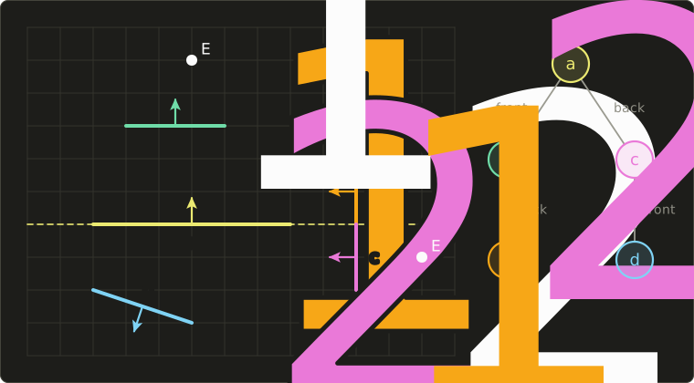
Traverse for the eye :
- At : has , front. So: back subtree, , front subtree.
- Back subtree, at : has , front. So: back of (empty), , front of , which is .
- Then .
- Front subtree, at : , front. So: back of , which is , then , then the empty front.
Drawing order: .
Check it against the picture: looks down from above, is nearest and drawn last, and , below , is drawn before which could cover it.
For every decision flips at (now back, ), at (back) and at (, back), and the order becomes .
The tree is the same for both eyes: only the traversal changes.
In practice
BSP trees suit static scenes: building the tree is expensive (the choice of roots decides how many splits happen), but traversal is a fast linear walk with one side test per node.
That's why id Software's Doom (1993) and Quake used BSP trees for their levels, combined with other tricks, and why level editors had a separate, slow "build BSP" step.
Traversing front to back instead of back to front is just as easy, which is useful with a Z-buffer (near things first, so far things fail the depth test early) and for culling.
Moving objects don't fit into a static tree and are drawn with a Z-buffer on top.
10.7 Area subdivision and the A-buffer
Warnock's algorithm
The area subdivision method (領域分割法), John Warnock's algorithm (1969), is a divide-and-conquer image-space method.
Take an area of the screen (at first the whole screen) and look at how each polygon relates to it:
- surrounding (取り囲む): the polygon covers the whole area,
- intersecting (交差する): the polygon covers part of the area and sticks out,
- contained (内包される): the polygon lies completely inside the area,
- disjoint (分離): the polygon doesn't touch the area.
The area is simple, and can be drawn directly, if one of these holds:
- No polygon touches it: fill it with the background.
- Exactly one polygon touches it (intersecting or contained): fill the background and draw that polygon's part.
- One polygon surrounds it and is nearer than all others in the area: fill the area with that polygon.
Otherwise, divide the area into four quarters and repeat for each.
At the size of one pixel, stop and take the polygon that is nearest at the pixel center.
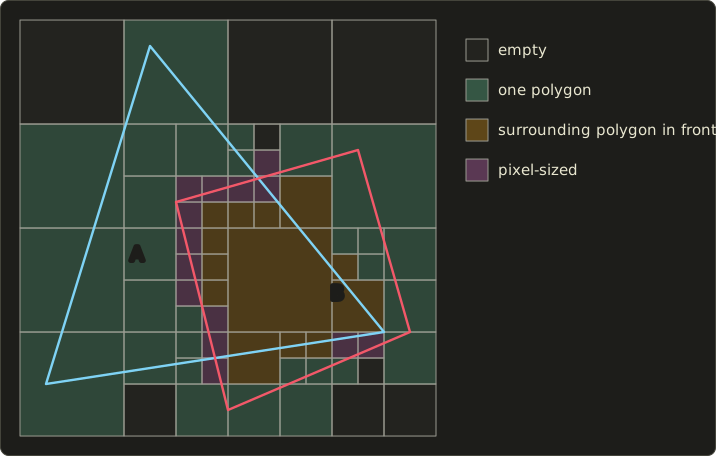
In the picture, quadrilateral B is in front of triangle A.
The 16×16 screen ends up as 64 areas instead of 256 pixels: 8 empty, 29 with a single polygon, 13 surrounded by B in front, and 14 pixel-sized ones where the edges of both polygons meet.
The work concentrates where the picture is complicated, and large simple regions are finished in one step.
The recursive division into four is a quadtree, the 2D cousin of the octree of chapter 9.
The A-buffer
The A-buffer (Aバッファ, Loren Carpenter, 1984) extends the Z-buffer instead: each pixel keeps a list of the surface fragments that touch it, each with its depth, color, opacity and a small bit mask saying which part of the pixel it covers.
When all polygons are drawn, every pixel sorts its list by depth and combines the fragments.
That solves two of the Z-buffer's weaknesses at once: partially covered pixels at edges are blended by their coverage (anti-aliasing), and semi-transparent surfaces are combined in the right order.
The price is memory that varies per pixel.
It was developed for Lucasfilm's REYES renderer, and today's GPU techniques for order-independent transparency with per-pixel lists follow the same idea (Part 2).
10.8 Comparing the methods
| Method | Space | Needs sorting? | Interpenetrating polygons | Transparency | Main cost |
|---|---|---|---|---|---|
| Depth sort (painter's) | object (sort), image (draw) | yes, by depth | must split | easy (back to front) | sorting, pair tests, splits |
| Z-buffer | image | no | handled per pixel | hard | one depth value per pixel |
| Scanline | image | edges by y and x | split the span | possible | bookkeeping per scanline |
| Ray casting | image | no (nearest hit) | handled | yes (continue the ray) | rays × objects, needs acceleration |
| BSP tree | object | no, the tree gives the order | split while building | easy (back to front) | building the tree; static scenes |
| Area subdivision (Warnock) | image | no | resolved at pixel level | hard | recursion where the image is complex |
| A-buffer | image | per pixel list | handled | yes | variable memory per pixel |
Exam points
- Back-face culling alone is complete hidden surface removal only for a single convex object.
- Object-space methods compare polygons (exact, up to pairs); image-space methods decide per pixel (precision of the pixel grid).
- The painter's algorithm draws back to front and overwrites; it fails for cyclic overlap and interpenetration unless polygons are split.
- The Z-buffer method: image space, no sorting, any drawing order, handles interpenetration, memory proportional to the number of pixels (not polygons); weak at transparency and anti-aliasing; limited precision causes z-fighting, worst far from the camera.
- The scanline method works with spans and needs only one scanline of depth; it uses coherence between neighboring scanlines.
- Ray casting takes the nearest intersection along the ray through each pixel.
- A BSP tree is built once and is view independent; the traversal draws the side away from the eye first.
- Warnock's algorithm subdivides the screen into four until each area is simple.
10.9 Light sources
Now the second question: how bright is a visible surface?
That depends on the light that reaches it, so first we need models of light sources (光源).
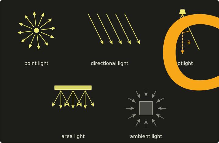
Point light
A point light (点光源) has a position and sends light equally in all directions, like a small bulb.
The direction to the light, , changes from point to point on a surface.
Physically, the light passing through a sphere around the source spreads over the sphere's area , so the light arriving at distance falls with the inverse square law:
Twice as far means a quarter of the light.
Real-time graphics traditionally used a more flexible attenuation (減衰) factor with three constants (OpenGL's old fixed-function lights had exactly these three):
is the constant, the linear and the quadratic attenuation.
, is the physical law; the extra terms keep the light from blowing up close to the source and let artists shape the falloff.
Example: , , and : .
Modern physically based engines use the plain inverse square law with a smooth cut-off radius.
Directional light
A directional light or parallel light (平行光源) has only a direction: all its rays are parallel, is the same at every point, and there's no attenuation.
It models a very distant source, the sun above all: the sun is about 150 million km away, so across a scene of a few kilometers its rays are parallel for every practical purpose.
It's the cheapest light to compute.
Spotlight
A spotlight (スポットライト) is a point light that shines only into a cone: it has a position, an axis direction and a cut-off angle .
Let be the angle between the axis and the direction from the light to the surface point, (with unit vectors, and pointing from the surface to the light).
Outside the cone () the light is zero.
Inside, a classic falloff (Warn's model) multiplies the light by , so the spot is brightest on its axis; a larger concentrates it more.
Many engines instead fade linearly in between an inner and an outer cone angle.
Example: and : .
With an inner angle of 20° and an outer angle of 30°, a point at gets of the light.
Area light
An area light (面光源) emits from a surface with a size: a window, a ceiling panel, a softbox in a photo studio.
A fluorescent tube is the 1D version, a linear light (線光源).
Because the light comes from many points at once, objects cast soft shadows with a gradual penumbra (chapter 11), and highlights on shiny objects take the shape of the light.
Offline renderers sample many points on the light; real-time engines use clever approximations (Part 2, and the GLSL series, chapter 10).
Ambient light
In reality, a surface facing away from every lamp is not black: light bounces off walls, floor and ceiling and reaches it indirectly.
Computing that properly is global illumination (chapter 12).
The cheap stand-in is ambient light (環境光): a constant amount of light that arrives from everywhere and lights every surface equally, regardless of its orientation.
It fills the shadows so they aren't pitch black, but it also makes them flat, because it ignores the shape completely.
10.10 Reflection models
A reflection model (反射モデル), also called a lighting or illumination model, gives the light leaving a surface point towards the eye, from the light arriving at it.
The classic local model has three parts: ambient, diffuse and specular.
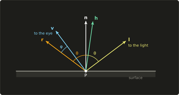
It uses five vectors at the surface point P:
- : the surface normal,
- : the direction from P to the light,
- : the direction from P to the eye (the viewer),
- : the mirror direction of about ,
- : the half vector between and .
All five are unit vectors; in this chapter I leave out the hats so the formulas stay readable.
The picture uses the numbers of the worked example below:
Colors are handled one channel at a time: every formula below is computed separately for R, G and B, and a product of two colors means multiplying their channels.
The coefficients , and are the material's reflectances (between 0 and 1 per channel), and and are the colors of the ambient light and of the light source.
Ambient reflection
Constant over the whole object.
Usually : a red object reflects red ambient light.
Diffuse reflection: Lambert's cosine law
A matte surface (paper, plaster, unpolished wood) scatters the light it receives in all directions: diffuse reflection (拡散反射).
How much light it receives depends on the angle between the normal and the light direction: a beam hitting the surface at a slant spreads over a larger area, so each square centimeter gets less.
That's Lambert's cosine law (ランバートの余弦則, Lambert, 1760), and with unit vectors the cosine is a dot product (Linear Algebra chapter 4 shows the picture):
The max removes light from behind the surface.
Why doesn't appear?
An ideal diffuse (Lambertian) surface looks equally bright from every direction.
Seen from a grazing angle, each pixel of the image covers a larger piece of the surface (foreshortening), but an ideal diffuse surface also sends less light per area towards grazing directions, in proportion to the cosine of the viewing angle, and the two effects cancel exactly.
So diffuse reflection is view independent: you can walk around a sheet of paper and it keeps its brightness.
This is also why radiosity (chapter 12) can precompute diffuse lighting once for all views.
Specular reflection: the Phong model
Shiny surfaces (plastic, polished metal, wet skin) also show specular reflection (鏡面反射), seen as a highlight (ハイライト): a bright spot where the light is reflected almost like a mirror towards the eye.
A perfect mirror reflects the light only into the mirror direction
which is the reflection formula of Linear Algebra chapter 4 applied to the incoming direction .
A real glossy surface spreads the reflection around .
Bui Tuong Phong (1975) modeled this spread with a power of the cosine of the angle between and :
The exponent is the shininess or specular exponent (鏡面反射指数, also ハイライト係数): a cosine below 1 raised to a large power drops quickly, so a large gives a small, sharp highlight (polished metal, in the hundreds) and a small a broad, soft one (rubber, around 5 to 10).
Specular reflection is view dependent: move your head and the highlight moves across the surface.
For plastics and other non-metals the highlight has the color of the light ( is gray); for metals it takes the color of the metal ( is colored, think of gold).
The specular term is only added when the light is in front of the surface ().
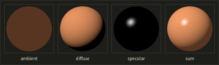
The Phong illumination equation
Adding the three terms and the attenuation of section 10.9 gives the Phong reflection model (フォンの反射モデル).
With several lights , each light adds its own diffuse and specular part, while the ambient part is counted once:
Summing works because light adds up linearly, which is also why this sum must be computed in linear values and only encoded to sRGB at the end (chapter 3, section 3.7).
If the result goes above 1 it's clipped, or, in HDR rendering, compressed by tone mapping (chapter 15).
A fully worked example
A point P on a floor is lit by one point light:
- P is at the origin, the floor's normal is .
- The light is at , with color (slightly warm) and attenuation , , .
- The eye is at .
- The ambient light is .
- The material: (orange), , .
Step 1: vectors.
To the light: , length , so and .
To the eye: , length , so .
Step 2: attenuation.
Step 3: diffuse factor.
Step 4: specular factor.
The eye is close to the mirror direction (), so the highlight is still at two thirds of its full strength.
Step 5: the three terms, per channel.
Step 6: sum.
A warm orange; encoded to 8-bit sRGB (chapter 3) it's about (198, 157, 129).
Notice how the colors combine: the diffuse part is the orange material times the warm light, while the highlight is gray times the light, so it has the light's color.
Under a pure blue light , the diffuse part would be : almost black, because the material reflects little blue.
Here is the model as a small C++ function, with the same numbers:
#include <algorithm>
#include <cmath>
#include <cstdio>
#include "linalg.hh"

// component-wise product: the color of the light times the color of the material
Vec3 mul(Vec3 a, Vec3 b) { return {a.x * b.x, a.y * b.y, a.z * b.z}; }

struct Material {
  Vec3 ka, kd, ks; // ambient, diffuse and specular reflection coefficients (RGB)
  float shininess; // the exponent alpha
};

struct PointLight {
  Vec3 position;
  Vec3 color;       // I_L
  float kc, kl, kq; // constant, linear and quadratic attenuation
};

// The Phong reflection model for one point light.
// p: surface point, n: unit normal, eye: eye position.
Vec3 phong(Vec3 p, Vec3 n, Vec3 eye, const Material &m, const PointLight &light, Vec3 ambient) {
  Vec3 toLight = light.position - p;
  float d = length(toLight);
  Vec3 l = toLight / d;                      // unit vector towards the light
  Vec3 v = normalize(eye - p);               // unit vector towards the eye
  float att = 1.0f / (light.kc + light.kl * d + light.kq * d * d);
  float nl = dot(n, l);
  Vec3 color = mul(m.ka, ambient);           // ambient term
  if (nl > 0) {                              // the light is in front of the surface
    Vec3 r = 2.0f * nl * n - l;              // mirror direction of l
    float spec = std::pow(std::max(dot(r, v), 0.0f), m.shininess);
    color = color + att * (nl * mul(m.kd, light.color) + spec * mul(m.ks, light.color));
  }
  return color;
}

int main() {
  Material m{{0.8f, 0.4f, 0.2f}, {0.8f, 0.4f, 0.2f}, {0.5f, 0.5f, 0.5f}, 10.0f};
  PointLight light{{0, 3, 4}, {1.0f, 0.9f, 0.8f}, 1.0f, 0.1f, 0.02f};
  Vec3 c = phong({0, 0, 0}, {0, 1, 0}, {0, 8, -6}, m, light, {0.2f, 0.2f, 0.2f});
  printf("I = (%.4f, %.4f, %.4f)\n", c.x, c.y, c.z);
  return 0;
}
I = (0.5662, 0.3376, 0.2210)Blinn–Phong: the half vector
Jim Blinn (1977) replaced with the angle between the normal and the half vector (ハーフベクトル, also 中間ベクトル), the direction exactly halfway between the light and the eye:
This is the Blinn–Phong model (ブリン・フォンの反射モデル).
If the normal points exactly along , the surface is a mirror that reflects the light straight into the eye, so the idea is the same.
In our example, with length , so and , an angle of about 8.1°.
That's half of : when , and lie in one plane, the angle between and is exactly half the angle between and .
So with the same exponent the Blinn–Phong highlight is larger: instead of 0.665.
To get about the same highlight, use roughly four times the exponent: , very close to Phong's 0.665.
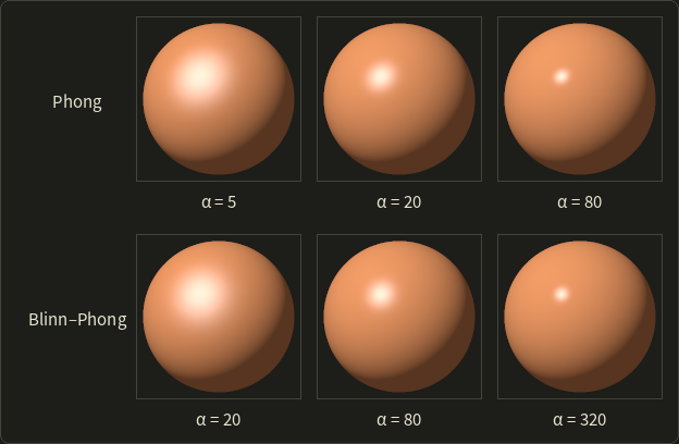
Blinn–Phong became the standard for three reasons.
With a directional light and a distant viewer, and are constant, so is computed once per frame instead of per point (the fixed-function lighting of OpenGL and Direct3D used the half vector).
Its highlights are stretched at grazing angles like real ones (think of the long reflection of the sun on a lake), while Phong's are always round.
And it's closer to the physically based microfacet models of chapter 12, which are also written with .
Limits of the classic model
The Phong model is an empirical model: it was made to look right, not derived from physics.
It doesn't conserve energy (nothing stops from reflecting more light than arrives, and a larger makes the highlight smaller without making it brighter), it has no Fresnel effect (surfaces become more mirror-like at grazing angles), and it only looks at one direct light path.
Modern renderers use physically based reflection with BRDFs (chapter 12 and Part 2), but the structure stays the same: a diffuse part, a specular part with a highlight around the mirror direction, a sum over lights.
You'll implement Phong lighting in the OpenGL series, chapter 10, with all three light types in chapter 12, and in shaders in the GLSL series, chapter 9.
10.11 Shading methods
The reflection model says how to light one point with one normal.
A polygon mesh only has normals at its vertices (or one per face), and millions of pixels in between.
A shading method (シェーディング手法) decides where the reflection model is evaluated and how the results fill the polygon.
There are three classics.
Flat shading
Flat shading or constant shading (フラットシェーディング, コンスタントシェーディング) evaluates the model once per polygon, with the polygon's face normal, and fills the whole polygon with that one color.
It's the cheapest, and exactly right for objects that really are flat-sided (a cube, a crystal) under a directional light and a distant viewer.
On a curved surface approximated by polygons, it shows every facet, and the eye's Mach bands (chapter 3) even exaggerate each step in brightness.
Gouraud shading
Gouraud shading (グーローシェーディング, Henri Gouraud, 1971), also called smooth shading, evaluates the model at the vertices and interpolates the colors across the polygon:
- Give each vertex a vertex normal (頂点法線), usually the average of the normals of the faces around it (chapter 9), so neighboring polygons share it.
- Compute the color at each vertex with the reflection model.
- Interpolate the colors linearly over the polygon: along the edges and then along each scanline in the classic version, or with barycentric coordinates (section 6.9) on a GPU.
Because neighboring polygons share the vertex colors, the brightness is continuous across edges, and the facets disappear.
It's cheap: a mesh has far fewer vertices than the pixels it covers.
Its weaknesses all come from computing light only at the vertices:
- Highlights are missed or smeared. A highlight smaller than a polygon that falls between the vertices is simply lost, because no vertex sees it. A highlight that falls on a vertex is spread over all the polygons around it, as a blurry star whose shape follows the mesh. When the object moves, the highlight flickers as it jumps from vertex to vertex.
- Mach bands. The brightness is continuous across an edge, but its slope changes there, and the eye adds bright and dark stripes along such slope changes (chapter 3), so the mesh structure can still show through.
Phong shading
Phong shading (フォンシェーディング, Phong, 1975) interpolates the normals instead of the colors and evaluates the reflection model at every pixel:
- Interpolate the vertex normals across the polygon.
- Normalize the interpolated normal at each pixel. A linear blend of unit vectors is shorter than 1, as we'll see in a moment, and the dot products of the model need unit vectors.
- Evaluate the reflection model with this normal.
The highlight now appears wherever it should, even in the middle of a large polygon, with the shape the light and the curvature give it, independent of the mesh.
The price is one evaluation of the reflection model per pixel instead of per vertex.
Don't mix up the names.
The Phong reflection model (section 10.10) is the formula with ambient, diffuse and ; Phong shading is the method that interpolates normals and lights every pixel.
They're independent: you can use the Phong model with Gouraud shading (the fixed-function GPUs did exactly that) or Phong shading with a completely different, physically based reflection model (every modern engine does).
Worked example: a highlight between two vertices
Take one edge of a mesh, whose two vertices have the normals
(both unit vectors: ), like two points on a curved surface on either side of its top.
The light and the eye are both straight in front: (a "headlight" setup).
We look at the diffuse factor and the specular factor with .
At the vertices.
.
, so and : no highlight at all.
The second vertex gives the same by symmetry.
Gouraud at the midpoint interpolates these results: diffuse , specular .
Phong at the midpoint interpolates the normals:
Now , , and : diffuse 1 and a full highlight, exactly where the surface faces the light, which Gouraud shading missed completely.
A quarter of the way from : the blend is with length , normalized .
Then , and with the mirror term is , so the specular factor is .
The highlight rises from almost 0 at a quarter to 1 in the middle: it is narrow and sits between the vertices.
And step 2 matters: without normalizing, the midpoint normal gives , no better than Gouraud.
(In fact the z component of every blend of these two normals is 0.8, so an unnormalized normal would give a flat 0.8 along the whole edge.)
The comparison, rendered
Here is a low-poly sphere (a UV sphere with 12 segments around and 8 from pole to pole, 168 triangles) rendered with each method, using the Phong reflection model of section 10.10 with and a directional light from the upper left.
The pictures were computed with a small software rasterizer that uses exactly the formulas of this chapter and chapter 6: edge functions, barycentric interpolation, a Z-buffer, then the shading method, and the linear results encoded to sRGB.
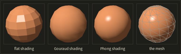
- Flat: every facet is visible, and the facet that faces the highlight direction lights up as a whole.
- Gouraud: smooth, but the highlight is gone. The mesh view on the right shows why: the highlight lies inside one quadrilateral, away from all of its vertices, and the vertices see only the dim edge of it.
- Phong: the highlight is where it belongs, round and sharp, although the silhouette is just as polygonal as before. Shading can hide facets inside the outline, not on it.
The plot shows the brightness along the image row through the center of the highlight:
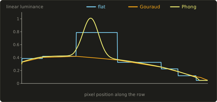
Flat shading is a staircase, with a jump at every edge.
Gouraud shading is continuous but made of straight pieces; the corners where the slope changes are exactly where Mach bands appear.
Phong shading is smooth and has the highlight peak that Gouraud never sees.
On a GPU: per vertex or per fragment
On a GPU the choice is simply where you call the reflection model:
- In the vertex shader and pass the color on: the rasterizer interpolates it, and you get Gouraud shading. The fixed-function pipelines of OpenGL 1.x and Direct3D up to version 9 worked this way (
glShadeModel(GL_SMOOTH);GL_FLATgave flat shading). - In the fragment shader, with the normal (and the position) passed on from the vertex shader: the rasterizer interpolates the normal, the fragment shader normalizes it and lights the pixel, and you get Phong shading. This is the norm today.
- Flat shading: mark the varying as not interpolated (
flatin GLSL,nointerpolationin Slang, as in HLSL); the whole triangle then uses the value of one of its vertices (the "provoking vertex").
The cost difference: a 1920×1080 image has about 2.07 million pixels (more fragments with overdraw), while a typical character has some tens of thousands of vertices.
Modern GPUs run billions of fragment shader invocations per second, so per-pixel lighting is cheap enough, and techniques like normal mapping (chapter 11) need it anyway.
Here is Phong shading with the Phong reflection model for one point light (attenuation left out to keep it short), as a fragment shader:
struct Scene {
  float3 lightPos;   // world space
  float3 lightColor; // I_L
  float3 ambient;    // I_a
  float3 eyePos;     // world space
  float3 kd;         // diffuse (and ambient) color of the material
  float3 ks;         // specular color
  float shininess;   // alpha
};
ConstantBuffer<Scene> scene;

float3 phongModel(float3 n, float3 l, float3 v) {
  float3 color = scene.kd * scene.ambient;
  float nl = dot(n, l);
  if (nl > 0.0) {
    float3 r = reflect(-l, n); // = 2 (n.l) n - l
    float spec = pow(max(dot(r, v), 0.0), scene.shininess);
    color += scene.lightColor * (scene.kd * nl + scene.ks * spec);
  }
  return color;
}

[shader("fragment")]
float4 fragmentMain(float3 worldPos : TEXCOORD0, float3 normal : NORMAL) : SV_Target {
  float3 n = normalize(normal); // interpolation made it shorter than 1
  float3 l = normalize(scene.lightPos - worldPos);
  float3 v = normalize(scene.eyePos - worldPos);
  return float4(phongModel(n, l, v), 1.0);
}
#version 450
layout(location = 0) in vec3 worldPos;
layout(location = 1) in vec3 normal;
layout(location = 0) out vec4 outColor;
layout(set = 0, binding = 0) uniform Scene {
vec3 lightPos; // world space
vec3 lightColor; // I_L
vec3 ambient; // I_a
vec3 eyePos; // world space
vec3 kd; // diffuse (and ambient) color of the material
vec3 ks; // specular color
float shininess; // alpha
};
vec3 phongModel(vec3 n, vec3 l, vec3 v) {
vec3 color = kd * ambient;
float nl = dot(n, l);
if (nl > 0.0) {
vec3 r = reflect(-l, n); // = 2 (n.l) n - l
float spec = pow(max(dot(r, v), 0.0), shininess);
color += lightColor * (kd * nl + ks * spec);
}
return color;
}
void main() {
vec3 n = normalize(normal); // interpolation made it shorter than 1
vec3 l = normalize(lightPos - worldPos);
vec3 v = normalize(eyePos - worldPos);
outColor = vec4(phongModel(n, l, v), 1.0);
}struct Scene {
float3 lightPos; // world space
float3 lightColor; // I_L
float3 ambient; // I_a
float3 eyePos; // world space
float3 kd; // diffuse (and ambient) color of the material
float3 ks; // specular color
float shininess; // alpha
};
ConstantBuffer<Scene> scene;
float3 phongModel(float3 n, float3 l, float3 v) {
float3 color = scene.kd * scene.ambient;
float nl = dot(n, l);
if (nl > 0.0) {
float3 r = reflect(-l, n); // = 2 (n.l) n - l
float spec = pow(max(dot(r, v), 0.0), scene.shininess);
color += scene.lightColor * (scene.kd * nl + scene.ks * spec);
}
return color;
}
float4 fragmentMain(float3 worldPos : TEXCOORD0, float3 normal : NORMAL) : SV_Target {
float3 n = normalize(normal); // interpolation made it shorter than 1
float3 l = normalize(scene.lightPos - worldPos);
float3 v = normalize(scene.eyePos - worldPos);
return float4(phongModel(n, l, v), 1.0);
}
All three languages have reflect(d, n) built in, which computes for an incoming direction ; we pass , the direction the light travels.
For Blinn–Phong, replace the two lines of the specular part with h = normalize(l + v) and pow(max(dot(n, h), 0.0), shininess), as in Linear Algebra chapter 4.
Moving the same phongModel call into the vertex shader and passing the color instead of the normal turns this into Gouraud shading.
10.12 Transparency
Glass, water, smoke and leaves let some of the light from behind them through.
The simplest model gives each surface an opacity (不透明度) between 0 (invisible) and 1 (opaque), usually stored as the fourth color channel, alpha.
(This has nothing to do with the shininess exponent; the letter is just popular.)
Alpha blending
When a surface with color and opacity is drawn over the color already in the frame buffer, alpha blending (アルファブレンディング) mixes them with the over operator (Porter and Duff, 1984):
That's a linear interpolation between what's behind and the new surface, done per channel by the blending stage of the GPU pipeline (section 6.5).
It depends on the order
Draw a red pane and a blue pane , both with , over a white background .
Red first, then blue:
Blue first, then red:
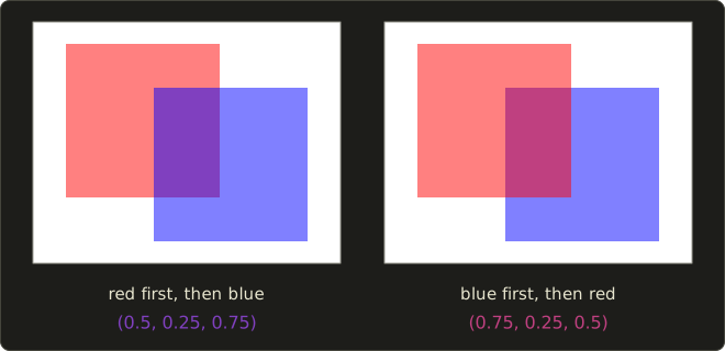
The pane drawn last dominates.
For a correct picture, the surface nearer the eye must be blended last, so transparent surfaces must be drawn back to front: the painter's algorithm again.
Transparency with a Z-buffer
That clashes with the Z-buffer, which happily draws in any order.
If a near glass pane is drawn first and writes its depth, an object behind it drawn later fails the depth test and disappears instead of showing through the glass.
The standard recipe:
- Draw all opaque objects first, in any order, with depth testing and depth writing on.
- Sort the transparent objects from back to front (by distance from the camera).
- Draw them with depth testing on (so opaque objects in front still hide them) and depth writing off (so they never hide each other or later objects).
The sorting is per object, so it has all the problems of section 10.2: intersecting or cyclically overlapping transparent objects come out wrong somewhere.
Exact solutions are order-independent transparency methods, such as the A-buffer of section 10.7 or depth peeling (Part 2).
One special case needs no sorting: additive blending, , is commutative (addition doesn't care about order), which is why fire, sparks and glows are usually drawn additively.
You'll set up blending in the OpenGL series, chapter 16.
Alpha blending only fades the background behind a surface; it doesn't bend it.
Real glass and water refract the light (Snell's law) and reflect more at grazing angles (the Fresnel effect); ray tracing handles both, in chapter 12.
Exam points
- Phong reflection model: ambient (constant), diffuse (Lambert, view independent), specular (view dependent), with .
- A larger shininess gives a smaller, sharper highlight. Blinn–Phong uses with the half vector; for a similar highlight.
- Light sources: point (position, inverse square falloff), directional (direction only, no falloff, the sun), spot (cone), area (soft shadows), ambient (constant, stands in for indirect light).
- Flat shading: one color per polygon. Gouraud: colors at the vertices, interpolated (cheap; highlights missed or smeared; Mach bands). Phong shading: normals interpolated and normalized, model evaluated per pixel.
- "Phong shading" (the interpolation method) and the "Phong reflection model" (the formula) are different things.
- Alpha blending with the over operator depends on the drawing order; transparent surfaces are drawn back to front after the opaque ones, with depth writes off.
10.13 Summary
- Hidden surface removal decides what is visible at each pixel. Object-space methods compare polygons; image-space methods work per pixel. Back-face culling alone is enough only for one convex object.
- The painter's algorithm (depth sort) draws back to front; cyclic overlap and interpenetration require splitting polygons.
- The Z-buffer method keeps a depth per pixel and draws in any order with a per-pixel depth test; it handles interpenetration but not transparency, and its precision falls with the square of the distance (z-fighting).
- The scanline method compares depths per span on one scanline at a time; ray casting finds the nearest hit along a ray per pixel; a BSP tree gives a back-to-front order for any eye position; Warnock's algorithm subdivides the screen until each area is simple; the A-buffer keeps a fragment list per pixel.
- Light sources: point (attenuation , physically ), directional, spotlight, area and ambient.
- The Phong reflection model sums ambient, diffuse () and specular () terms over the lights, per color channel; Blinn–Phong uses the half vector.
- Flat shading lights once per polygon, Gouraud shading lights the vertices and interpolates colors, Phong shading interpolates normals and lights every pixel.
- Alpha blending is order dependent: opaque first, then transparent back to front.
10.14 Key terms
| English | 日本語 |
|---|---|
| hidden line removal | 隠線消去 |
| hidden surface removal | 隠面消去 |
| object-space method | 物体空間法(オブジェクト空間法) |
| image-space method | 画像空間法 |
| depth sort method | 奥行きソート法 |
| painter's algorithm | 画家のアルゴリズム |
| cyclic overlap | 循環する重なり |
| Z-buffer method | Zバッファ法 |
| depth buffer, Z-buffer | 深度バッファ、Zバッファ |
| depth test | 深度テスト |
| z-fighting | Zファイティング |
| scanline method | スキャンライン法 |
| span | スパン |
| ray casting | レイキャスティング法 |
| BSP tree | BSP木(BSP法) |
| area subdivision (Warnock's algorithm) | 領域分割法(ウォーノックのアルゴリズム) |
| A-buffer | Aバッファ |
| light source | 光源 |
| point light | 点光源 |
| directional (parallel) light | 平行光源 |
| spotlight | スポットライト |
| area light | 面光源 |
| linear light | 線光源 |
| ambient light | 環境光 |
| attenuation | 減衰 |
| reflection model | 反射モデル |
| diffuse reflection | 拡散反射 |
| Lambert's cosine law | ランバートの余弦則 |
| specular reflection | 鏡面反射 |
| highlight | ハイライト |
| shininess (specular exponent) | 鏡面反射指数(ハイライト係数) |
| Phong reflection model | フォンの反射モデル |
| half vector | ハーフベクトル(中間ベクトル) |
| Blinn–Phong model | ブリン・フォンの反射モデル |
| shading | シェーディング |
| flat (constant) shading | フラットシェーディング(コンスタントシェーディング) |
| Gouraud shading | グーローシェーディング |
| Phong shading | フォンシェーディング |
| vertex normal | 頂点法線 |
| opacity | 不透明度 |
| alpha blending | アルファブレンディング |
10.15 Challenges
- ★ A 3840×2160 screen uses a 32-bit depth buffer. How many bytes is it, and how many MiB? With a 24-bit depth buffer, and , estimate the smallest depth difference that can still be resolved at a distance of 50 m, and again with .
- ★ A directional light with color comes from , the normal is and the eye is in the direction . With , , and , compute , all three terms and the final color. Then replace the specular term with Blinn–Phong and and compare.
- ★★ Using the segments of section 10.6, give the BSP drawing order for the eye . Then build the tree again with as the root (inserting , , in this order) and check that it gives the same orders for and as the tree in the chapter.
- ★★ Two vertices of an edge have the normals and , and with . Compute the specular factor at the vertices and at the midpoint with Gouraud shading and with Phong shading, and the length of the interpolated normal before normalizing.
- ★★★ Three glass panes with (red, green, blue) are blended over black. Show with numbers that two different drawing orders give different results, but that additive blending gives the same result in any order. Then explain why sorting transparent objects by their centers can still fail, using a picture like the cyclic overlap of section 10.2.
Multiple choice
Q1 ★ Which of the following statements about the Z-buffer method is correct?
| A | The polygons must be sorted by depth before they are drawn. |
| B | It draws semi-transparent polygons correctly in any order. |
| C | It is an object-space method that compares every pair of polygons. |
| D | The memory it needs grows with the number of polygons in the scene. |
| E | It resolves polygons that pass through each other pixel by pixel, without splitting them. |
Q2 ★ Which of the following statements about shading methods is correct?
| A | Gouraud shading computes colors at the vertices and interpolates them, so a highlight that falls inside a polygon, away from its vertices, can be lost. |
| B | Gouraud shading interpolates the normal vectors across the polygon and evaluates the reflection model at every pixel. |
| C | Phong shading computes one color per polygon from the face normal. |
| D | Phong shading and the Phong reflection model are two names for the same thing. |
| E | Flat shading hides the polygon edges of a curved surface completely. |
Q3 ★★ At a surface point, , the direction to the light is and the direction to the eye is . The light's intensity is 1, and . What is the specular term of the Phong reflection model?
| A | 0.18 |
| B | 0.32 |
| C | 0.4608 |
| D | 0.48 |
| E | 0.9216 |
10.16 Practical assignment
Z-buffer and shade a tiny scene on graph paper.
You need graph paper, a ruler, red and blue pencils and a calculator.
You'll do by hand what a GPU does for every frame: decide visibility with a Z-buffer, compare it with the painter's algorithm, and shade one triangle in three ways.
The screen is 8×6 pixels, with pixel covering the square from to and its center at (y up).
- Triangle P: , , with depths 0.2, 0.6, 0.2. Its depth plane is .
- Triangle Q: , , with depth 0.4 at all three vertices.
- Coverage. Draw the grid and both triangles. For every pixel center decide whether it lies in P, in Q or in both (use the edge functions of chapter 6, or the line equations of the edges; no center lies exactly on an edge). Mark the pixels covered by both.
- Depths. Write into every pixel covered by P, and 0.4 into every pixel covered by Q. Where do the two triangles pass through each other?
- Z-buffer, two orders. Start with all depths at 1. Draw P then Q with the depth test, writing the winning color and depth into a second grid. Then do it again in the order Q then P in a third grid. Color the results.
- Painter's algorithm. Sort P and Q by their average vertex depth and paint them back to front, overwriting, into a fourth grid. Count the pixels where the result differs from the Z-buffer, and explain why with the line of step 2.
- Shade the vertices. Give P the vertex normals , , , and use a gray material with , , , , a white light of intensity 1 and . Compute the intensity at A, B and C (with , ).
- Flat, Gouraud and Phong. For flat shading, use the normalized sum of the three vertex normals as the face normal and compute one intensity for the whole triangle. For the pixel centers and , compute the barycentric coordinates with respect to A, B, C (here simply , , ), then the Gouraud intensity (interpolate the three vertex intensities) and the Phong intensity (interpolate the normals, normalize, evaluate the model).
- Compare. Make a small table of flat, Gouraud and Phong for the two pixels and describe what happens to the highlight that sits exactly at vertex A.
How to check yourself:
- The grids of step 3 are identical: the Z-buffer doesn't care about the order. Inside the overlap, P wins exactly where and Q where .
- Step 4 differs from step 3 in only a few pixels, all in the overlap and all to the right of .
- In step 5, A gets the full highlight and B and C get almost none; all intensities lie between 0.1 and 1.0.
- In step 6, each set of barycentric coordinates adds up to 1, every normalized normal has length 1 (check with ), and every Gouraud value lies between the smallest and the largest vertex intensity.
コメント(0)
まだコメントはありません。
ログインするとコメント出来ます。