9. Polygon Meshes, Volumes and Other Shape Representations
Chapter 7 described solids and their boundaries, and chapter 8 built smooth curves and surfaces from control points.
In this chapter we meet the representations that real software mostly stores and draws: polygon meshes, the subdivision surfaces that make them smooth, voxels and octrees for things that have an inside (a CT scan, a sculpt, a destructible game world), implicit surfaces like metaballs, and a group of "other" representations that are generated rather than modeled by hand: fractals, L-systems, particles and point clouds.
Why does this matter?
Every GPU draws triangles, so whatever a shape started as, it usually ends up as a triangle mesh, and the mesh's layout decides how much memory and time it costs.
And many shapes are much easier to describe in another form first: a brain in a CT scan is a grid of numbers, a cloud of smoke is thousands of particles, a tree is a short rewriting rule.
For the exam, this chapter covers the last three syllabus items of area 3 (modeling): polygon surfaces (ポリゴン曲面の表現), volume-based shape representation (ボリュームを用いた形状表現) and other shape representations (そのほかの形状表現法).
There are many topics, so I'll keep each one tight and give every one a small worked example.
9.1 Polygon surfaces
A polygon mesh (ポリゴンメッシュ) is a surface made of flat polygons that share vertices and edges.
A curved surface becomes a polygon surface (ポリゴン曲面) by sampling points on it and connecting them: the more polygons, the closer the approximation.
Chapter 7 covered how a mesh's topology is stored and checked (B-rep, the half-edge structure, Euler's formula); here we look at the mesh as data for drawing.
Why triangles
Almost all real-time rendering uses triangles, for three reasons:
- Always flat. Three points always lie in one plane, so a triangle has one well-defined normal. A quad whose four corners don't lie in one plane (a non-planar quad) has no single normal, and it can be drawn differently depending on how it's split.
- Always convex and simple. Rasterization with edge functions and barycentric interpolation (chapter 6, section 6.9) works for every triangle without special cases.
- Everything else can be split into triangles. A convex polygon with vertices splits into triangles (a fan from one vertex); any simple polygon can be triangulated too.
Modeling tools still let you work with quads and n-gons (they're nicer for editing and for subdivision, section 9.2), and they triangulate when exporting or drawing.
Indexed meshes: vertex buffer and index buffer
The naive way to store a mesh is a list of triangles, each with its three corner positions written out in full: a polygon soup.
But in a closed mesh every vertex is shared by about six triangles, so most data is stored six times.
An indexed mesh (インデックス付きメッシュ) stores each vertex once in a vertex buffer (頂点バッファ) and describes the triangles as triples of vertex numbers in an index buffer (インデックスバッファ):
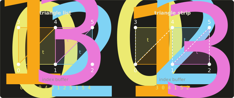
A "vertex" here means everything the GPU needs per corner, not just the position: typically a position (3 floats, 12 bytes), a normal (12 bytes) and texture coordinates (2 floats, 8 bytes), so 32 bytes per vertex.
Each triangle in the left picture lists its corners counter-clockwise, so all of them face us (section 6.4 explained why the winding matters).
Worked example. A terrain of 100 × 100 squares, each split into two triangles:
- vertices: ; triangles: .
- Polygon soup: corners of 32 bytes = bytes.
- Indexed, 32-bit indices: bytes of vertices plus bytes of indices = bytes, about 29% of the soup.
- Indexed, 16-bit indices: allowed because , so the indices take bytes and the total is bytes, about 23%.
Sharing vertices also saves work: the GPU keeps recently transformed vertices in a small cache, so a vertex shared by six triangles is often transformed only once.
For a closed triangle mesh without holes, Euler's formula from chapter 7 gives (exactly for a sphere-like mesh), which is where the "about six triangles per vertex" comes from: corners over vertices is about 6.
Triangle strips and fans
Even an index buffer repeats a lot: neighboring triangles share two vertices.
A triangle strip (トライアングルストリップ) lists the vertices so that every new vertex forms a triangle with the two before it.
triangles need only indices instead of .
In the right picture, the six indices 3, 0, 4, 1, 5, 2 give four triangles.
Triangle uses the vertices , but every second triangle would then come out clockwise, so for odd the GPU takes them in the opposite order.
Here that gives the triangles 3 0 4, 4 0 1, 4 1 5 and 5 1 2: all counter-clockwise.
A triangle fan (トライアングルファン) shares one center vertex: , perfect for a convex polygon or a disk.
For our 100 × 100 terrain, one strip per row of squares needs indices, and 100 rows need , a third of the list indices.
Rows can be joined into one long strip with a special primitive restart index (or with zero-area "degenerate" triangles).
Today, indexed triangle lists are the default in practice: with the vertex cache they're about as fast, and they're simpler to generate and process.
You'll build vertex and index buffers yourself in the OpenGL series, chapter 4.
Face normals and vertex normals
A face normal (面法線) is the normal of one flat polygon, the cross product of two of its edges (Linear Algebra chapter 5).
If every triangle is lit with its own face normal, the mesh looks faceted: you see every triangle (flat shading, chapter 10).
To make a polygon surface look like the smooth surface it approximates, each vertex gets a vertex normal (頂点法線): an average of the normals of the faces around it, which the renderer then interpolates across each triangle (chapter 10 covers Gouraud and Phong shading).
There are three common ways to average:
- Unweighted: normalize each face normal, add them up, normalize the sum.
- Area-weighted: add the unnormalized cross products. Their lengths are twice the triangle areas, so big faces count more, and there's one fewer normalization.
- Angle-weighted: weight each normalized face normal by the angle of that face at the vertex. This doesn't change when a face is split into more triangles, so it depends least on how the surface was triangulated.
Worked example. The vertex sits on the left edge of a table top (y is up, as everywhere in this series).
Triangle 1 is part of the top: , , .
Triangle 2 is part of the left side: , , .
So the top faces with area , and the side faces with area .
The corner angle of triangle 1 at V is 90° (), and of triangle 2 it's the angle between and : rad (26.6°).
| Method | Sum | Normalized | Tilt from +y |
|---|---|---|---|
| unweighted | 45° | ||
| area-weighted | 26.6° | ||
| angle-weighted | 16.4° |
Three methods, three different normals, and none is "the" right one: the vertex sits on a sharp edge, where no single normal is right.
Which brings us to hard edges.
Hard edges and smoothing groups
Averaging is right where the real surface is smooth and wrong where it has a crease, like the edge of a table or a box.
The fix is to split the vertex: store the same position twice (or more), each copy with the normal of its own side.
The renderer then sees two separate vertices, and the lighting has a crisp edge, a hard edge (ハードエッジ).
Modeling tools let you mark edges as hard or soft, or put faces into smoothing groups (スムージンググループ): normals are averaged only over faces of the same group.
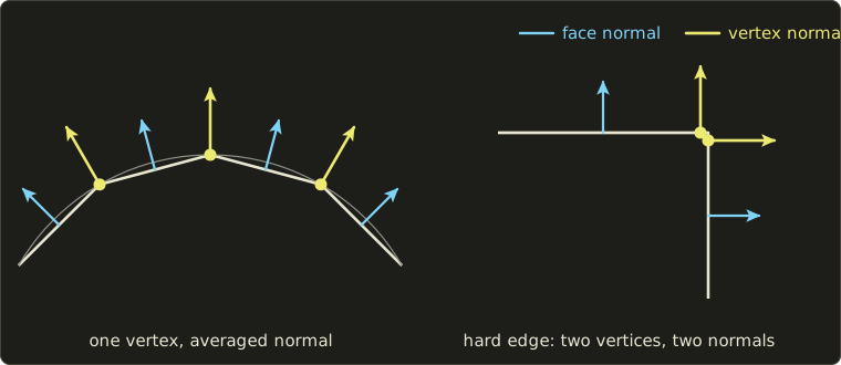
Worked example: the cube. A cube has 8 corners, but each corner touches 3 faces with 3 different normals.
Drawn with flat sides it needs vertices (4 per face), plus indices: bytes with 16-bit indices.
With only 8 shared vertices it would take bytes, but the averaged normals point diagonally out of the corners and the cube would be shaded like a blob.
The same splitting happens at texture seams: where a texture's UV layout is cut open, a vertex needs two different texture coordinates, so it's stored twice.
That's why a real mesh usually has noticeably more vertices than "corner positions".
Mesh quality
Not every set of triangles is a good mesh.
Problems worth knowing:
- Non-manifold parts (an edge shared by three or more faces, two solids touching at a single vertex) and holes break algorithms that expect a closed surface, from 3D printing to the inside tests of chapter 7.
- Inconsistent winding: some triangles listed clockwise, some counter-clockwise, so back-face culling removes the wrong ones and normals point inwards.
- T-junctions: a vertex lying on the middle of another triangle's edge. After rounding, the two sides of the edge no longer match exactly and pixel-sized cracks appear.
- Slivers: very thin, long triangles. They interpolate badly, cause shading artifacts, and are bad for simulations; meshing tools try to keep triangles close to equilateral.
- Too many or too few triangles: detail should go where the surface curves, not into flat areas.
Level of detail (LOD)
A building 1 km away covers a few dozen pixels; drawing all of its 100,000 triangles there is wasted work, and triangles smaller than a pixel also alias badly.
Level of detail (詳細度, LOD) means keeping several versions of a model and choosing by distance or by projected size:
- Discrete LOD: a handful of versions (for example 20,000, 5,000, 1,250 and 300 triangles), switched at thresholds. The switch can be seen as a sudden jump called popping (ポッピング); renderers hide it by blending the two versions for a moment (cross-fading) or by moving vertices smoothly into their new positions (geomorphing).
- Continuous LOD: the mesh can be coarsened or refined one small step at a time, for example with Hoppe's progressive meshes (1996), so there is no visible jump. Terrain renderers also refine locally: fine near the camera, coarse far away.
Worked example. How big is a sphere of radius m on a 1080-pixel-high screen with a 60° vertical field of view?
At distance , the visible height is and the sphere's diameter is 2, so its height in pixels is
At 10 m that's about 187 pixels, at 100 m about 18.7 pixels.
At 100 m the sphere covers about pixels, so a 20,000-triangle version would put about 73 triangles into every pixel: an obvious case for a 300-triangle LOD.
Engines choose the LOD from exactly this projected size, often expressed as the fraction of the screen height an object's bounding sphere covers.
Mesh simplification
Where do the coarse versions come from?
Mesh simplification (メッシュの簡略化) reduces the triangle count while keeping the shape:
- Vertex clustering: lay a grid over the model and merge all vertices in a cell into one. Fast and robust, but it ignores the shape and can change the topology.
- Vertex removal: remove a vertex and re-triangulate the hole it leaves.
- Edge collapse (エッジ縮約): pull the two ends of an edge together into one vertex. In the middle of a closed triangle mesh, one collapse removes 1 vertex, 3 edges and 2 triangles (the two triangles that shared the edge disappear and two pairs of edges merge), so stays the same. Going from 20,000 to 5,000 triangles takes collapses.
The art is in choosing which edge to collapse next and where to put the new vertex.
The standard answer, the quadric error metric (QEM) of Garland and Heckbert (1997), measures how far the new vertex would be from the planes of the original faces; we'll derive it in Part 2 of this series.
Recording the collapses in order, and their inverses (vertex splits), gives exactly the progressive mesh of the previous section.
Mesh file formats
Four formats are worth knowing, each with a different purpose:
| Format | Stores | Typical use |
|---|---|---|
| OBJ (Wavefront) | text; positions v, texture coordinates vt, normals vn, faces f (polygons allowed); materials in a separate .mtl file |
exchange between modeling tools |
| PLY (Stanford) | text or binary; a header declares the elements (vertex, face) and their properties, e.g. per-vertex color | 3D scanning, research data |
| STL | triangles only, each with a facet normal and its 3 corners written out; no shared vertices, colors, textures or units | 3D printing (from stereolithography) |
| glTF 2.0 (Khronos) | JSON scene description plus binary buffers (.gltf + .bin, or one .glb): meshes with index buffers, PBR materials, textures, node hierarchy, skins and animations |
delivering 3D assets to real-time engines and the web |
A tiny OBJ file, a unit square made of two triangles (note that OBJ counts vertices from 1):
# square.obj
v 0 0 0
v 1 0 0
v 1 1 0
v 0 1 0
vn 0 0 1
f 1//1 2//1 3//1
f 1//1 3//1 4//1
A face corner is written position/texcoord/normal, and an empty middle field means "no texture coordinate".
STL's binary layout is simple enough to compute a file size by hand: an 80-byte header, a 4-byte triangle count, then 50 bytes per triangle (12 floats for the normal and three corners = 48 bytes, plus a 2-byte attribute field).
Our 20,000-triangle terrain is bytes, about the size of the polygon soup, because STL is a polygon soup.
glTF 2.0 was released by Khronos in 2017 and became the international standard ISO/IEC 12113 in 2022; it stores exactly the vertex and index buffers of this section, ready to upload to the GPU.
You'll read glTF files yourself in the OpenGL series, chapter 13.
In code: area-weighted vertex normals
Using the linalg.hh header from the Linear Algebra series, the area-weighted normals are one loop: add each triangle's raw cross product to its three vertices, then normalize.
#include <cstdio>
#include <vector>
#include "linalg.hh"

// Area-weighted vertex normals: add each triangle's unnormalized face normal
// (its length is twice the triangle's area) to its three vertices, then normalize.
std::vector<Vec3> vertexNormals(const std::vector<Vec3> &pos, const std::vector<unsigned> &idx) {
  std::vector<Vec3> n(pos.size(), Vec3{0, 0, 0});
  for (size_t t = 0; t + 2 < idx.size(); t += 3) {
    unsigned a = idx[t], b = idx[t + 1], c = idx[t + 2];
    Vec3 fn = cross(pos[b] - pos[a], pos[c] - pos[a]);
    n[a] = n[a] + fn;
    n[b] = n[b] + fn;
    n[c] = n[c] + fn;
  }
  for (Vec3 &v : n) v = normalize(v);
  return n;
}

int main() {
  // the table edge of section 9.1: V, A, B on the top, D on the side
  std::vector<Vec3> pos = {{0, 0, 0}, {2, 0, 0}, {0, 0, -2}, {0, -1, -2}};
  std::vector<unsigned> idx = {0, 1, 2, 0, 2, 3};
  std::vector<Vec3> n = vertexNormals(pos, idx);
  printf("normal at V: (%.3f, %.3f, %.3f)\n", n[0].x, n[0].y, n[0].z);
  return 0;
}
normal at V: (-0.447, 0.894, 0.000)
The result is the area-weighted row of the table.
Remember that these normals are in object space: after a non-uniform scale they must be transformed with the inverse transpose, as in chapter 5, section 5.4.
9.2 Subdivision surfaces
The idea
Chapter 8 built smooth surfaces from rectangular grids of control points, but a character's head isn't a rectangle: patches have to be stitched together, and keeping the seams smooth is painful.
A subdivision surface (細分割曲面) starts instead from an ordinary coarse polygon mesh, the control mesh or cage (制御メッシュ), of any shape and topology, and refines it again and again by fixed rules.
Each step adds new vertices, moves the old ones a little, and the meshes converge to a smooth limit surface (極限曲面).
Schemes come in two families:
- approximating (近似型): the old vertices move, and the limit surface does not pass through the cage's vertices (Catmull–Clark, Loop, Doo–Sabin),
- interpolating (補間型): the old vertices stay where they are, and the surface passes through them (for example the butterfly scheme).
Catmull–Clark subdivision
The Catmull–Clark scheme (カトマル・クラーク法, 1978) is the standard in film and modeling tools.
It works on any polygon mesh, and after one step every face is a quad.
One step computes three kinds of new points:
- Face point (面点) for every face: the average of the face's vertices.
- Edge point (辺点) for every edge: the average of the edge's two endpoints and the face points of its two adjacent faces.
- Vertex point for every old vertex with valence (価数, the number of edges meeting there): the old vertex moves to
where is the average of the face points of the faces around and the average of the midpoints of the edges around it.
Then each old face with sides is replaced by quads, each made of one moved vertex, the two edge points next to it, and the face point.
Worked example: a cube with corners at .
- Face point of the face : the average of its four corners is . The six face points are , , .
- Edge point of the edge from to : its faces are and , with face points and , so the edge point is .
- Vertex point of , valence : ; the midpoints of its three edges are , , , so ; and with the old position drops out:
The corner has been pulled in strongly, from a distance of from the center to about , while the face points stay at distance 1: the cube is on its way to becoming round.
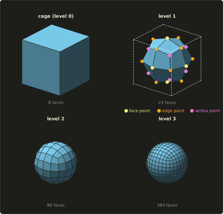
The counts after each step: 8 vertices, 12 edges and 6 faces become vertices, 48 edges and 24 quads, then 98, 192, 96 and 386, 768, 384.
Euler's formula still holds at every level (), and the face count is multiplied by 4 per step, so subdivision is something you do only a few levels deep.
Extraordinary vertices
On a regular quad grid every vertex has valence 4, and there Catmull–Clark reproduces exactly the uniform bicubic B-spline surface of chapter 8: the limit is smooth with continuous curvature ().
A vertex with any other valence is an extraordinary vertex (特異頂点, エクストラオーディナリー頂点): the cube's 8 corners have valence 3.
Edge points always get valence 4, and a face point gets the valence of its face's number of sides, so a triangle or a pentagon in the cage creates one more extraordinary vertex in the first step.
From then on all faces are quads and every new vertex has valence 4, so the number of extraordinary vertices stays fixed; they just become more and more isolated, and at those points the limit surface is only tangent-continuous ().
That's why modelers prefer "all-quad" cages with few extraordinary vertices, placed where they do no harm.
Boundaries and creases
At a boundary edge (an edge with only one face), the edge point is just the edge's midpoint, and a boundary vertex moves to using only its two boundary neighbors: the boundary becomes a cubic B-spline curve.
The same rules applied to edges inside the mesh that are tagged as creases (クリース) give sharp edges where the designer wants them, and Pixar's semi-sharp creases use the sharp rules for the first few steps only, for edges that are sharp from afar but slightly rounded up close.
Loop subdivision
The Loop scheme (ループ法, Charles Loop, 1987) is the triangle counterpart.
Each triangle is split into four by inserting a new vertex on every edge:
- Edge (odd) vertex: for an edge from to whose two triangles have the opposite vertices and , the new vertex is .
- Old (even) vertex of valence with neighbors : , with Loop's original ; a popular simpler choice (Warren's) is for and for .
For the regular valence 6 both give : Loop's formula gives , and .
Worked example. A spike: with six neighbors on the unit circle in the plane (their sum is ).
Then : the spike is smoothed down.
And an edge from to with opposite vertices and gets the new vertex .
Regular vertices of a triangle mesh have valence 6, other valences are extraordinary, and the limit is except at extraordinary vertices (), just like Catmull–Clark.
Doo–Sabin and others
The Doo–Sabin scheme (ドー・サビン法, 1978, the same year as Catmull–Clark) is a "dual" scheme: for every vertex of every face it creates a new point inside that face (in its simplest form, the average of the vertex, the two neighboring edge midpoints and the face point; for a quad this gives the weights for the vertex, for each neighbor and for the opposite corner, exactly Doo and Sabin's), then builds a new face from each old face, each old edge and each old vertex.
On a regular grid it gives biquadratic B-splines (only ).
The butterfly scheme is the best-known interpolating scheme: old vertices stay put, and each new edge vertex is computed from eight neighbors in a butterfly-shaped stencil.
In practice
Pixar's short film Geri's Game (1997) was the first Pixar production to use subdivision surfaces for a character, and Pixar released its implementation as the open-source library OpenSubdiv in 2012.
Today most modeling tools have it built in (in Blender, for example, the Subdivision Surface modifier is Catmull–Clark), and artists model a low-poly cage and let the software subdivide it.
Games usually subdivide offline and ship the result as an ordinary mesh with LODs, or use GPU tessellation, which the GLSL series, chapter 15 touches on.
9.3 Volume-based shape representation
A mesh describes only the surface.
For medical scans, sculpting, fluids or a game world you can dig into, we need to know what is inside, everywhere.
Voxels
A voxel (ボクセル, "volume element") is the 3D counterpart of a pixel: a small cube in a regular 3D grid, storing a value.
Storing a solid by marking which voxels it occupies is the spatial occupancy enumeration (ボクセル表現, literally 空間占有列挙) of chapter 7.
Voxels make some things trivial: the inside test is one array lookup, and CSG operations (union, intersection, difference) are just OR, AND and AND NOT per voxel.
The price is memory, which grows with the cube of the resolution:
- voxels.
- 1 bit each (inside or outside): bytes = 16 MiB.
- 1 byte each: 128 MiB. A 16-bit value each, as in CT data: 256 MiB.
- Doubling the resolution to multiplies all of these by 8: 2 GiB for the 16-bit grid.
And a voxel model is blocky unless the grid is very fine: a voxel grid is a sampled image, with all the aliasing of chapter 2.
Octrees
Most voxels of a typical object are either deep inside or far outside, and storing millions of identical "full" or "empty" cells is wasteful.
An octree (八分木, オクトツリー) stores the space adaptively.
Start with one cube around everything (the root), and classify each cube as
- full (entirely inside the object): a leaf,
- empty (entirely outside): a leaf,
- partial (on the boundary): split it into 8 equal child cubes (halving each axis) and classify those,
down to a maximum depth, where the remaining partial cubes are treated as full or empty (or keep a value, like a voxel).
The 2D version, with 4 children per square, is the quadtree (四分木).
Worked example. The domain is the cube and the object is the box (a box in one corner), with a maximum depth of 3 (unit voxels).
- Depth 0: the root is partial, so split it into 8 cubes of size 4.
- Depth 1: the cube is completely inside: 1 full leaf. The other 7 cubes each overlap the box partly (each has at least one axis in , where the box covers only ), so all 7 are split into cubes of size 2.
- Depth 2: in each of those 7 cubes, a child is inside when it lies in on every axis that was in . A cube with one such axis has 4 full and 4 empty children; with two such axes, 2 full and 6 empty; with all three (the cube ), 1 full and 7 empty. There are 3, 3 and 1 of these cubes, so full and empty leaves. All are decided, so depth 3 is never reached.
Total: nodes, of which 57 are leaves (20 full, 37 empty).
Check the volume: .
A plain voxel grid at the same resolution has cells.
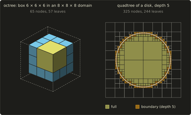
The right half shows why octrees pay off for curved shapes: the quadtree of a disk at depth 5 (the resolution of a grid, 1,024 cells) needs 325 nodes, and the small cells crowd only along the boundary.
In general the number of octree nodes grows with the object's surface area, roughly with the square of the resolution, while a voxel grid grows with the cube.
Octrees (and their relatives, sparse voxel structures and bounding volume hierarchies) are also used to speed up searches in space: ray tracing, collision detection and the view-frustum culling of chapter 6.
Volume data from CT and MRI
The biggest source of real volume data is medicine.
A CT scanner (X-ray computed tomography) measures, slice by slice, how strongly each small volume absorbs X-rays, in Hounsfield units (air about −1000, water 0, bone several hundred and more); a typical slice is samples, stored as 16-bit integers.
MRI (magnetic resonance imaging) measures signals from hydrogen nuclei and shows soft tissue well.
Stacking hundreds of slices gives a 3D grid of scalar values, a volume in exactly the voxel sense, often with a larger spacing between slices than between samples in a slice (anisotropic voxels).
Science and engineering produce the same kind of data from simulations: temperature, density or pressure on a 3D grid.
Such a grid has no surface yet.
To get a mesh, we extract the surface where the value crosses a threshold: an isosurface (等値面).
Marching squares: isolines in 2D
The 2D version is easiest to follow, so let's work through it fully.
Given a grid of samples and an iso value (しきい値) , we want the curve (an isoline, 等値線, like a contour line on a map).
The marching squares algorithm (マーチングスクエア法) handles one square cell at a time:
- Mark each corner as inside () or outside ().
- Combine the four marks into a 4-bit case number: bottom-left = 1, bottom-right = 2, top-right = 4, top-left = 8.
- Look the case up in a table that says which edges the curve crosses and how to connect them.
- Place each crossing point on its edge by linear interpolation: on an edge from with value to with value ,
There are cases:
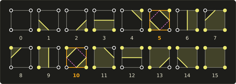
Worked example. A 4 × 4 grid of samples, iso value (rows listed from the top, , down to ):
| 3 | 1 | 1 | 3 | 2 |
| 2 | 1 | 9 | 7 | 3 |
| 1 | 3 | 7 | 6 | 2 |
| 0 | 1 | 3 | 2 | 0 |
The inside samples are the four middle ones: 9, 7, 7 and 6.
The cell with its bottom-left corner at has only its top-right corner inside, so it is case 4; the middle cell has all four corners inside, case 15 (no curve); and so on around the ring: 4, 12, 8 along the bottom, 6, 15, 9 in the middle row, 2, 3, 1 along the top.
Every edge that connects an inside and an outside sample gets a crossing point:
| Edge | Values | Crossing | |
|---|---|---|---|
| 3 → 7 | |||
| 3 → 7 | |||
| 2 → 6 | |||
| 6 → 2 | |||
| 7 → 3 | |||
| 7 → 3 | 0.5 | ||
| 9 → 1 | |||
| 1 → 9 |
Each cell connects its two crossings, and the eight segments join into one closed curve:
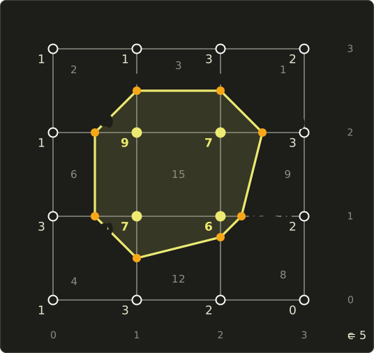
Notice that is only a quarter of the way from the sample 6, because 6 is barely above 5: interpolation puts the curve where the values say it is, instead of always at the edge midpoints, which is what makes the result smooth.
The ambiguous cases. In cases 5 and 10 the two inside corners sit diagonally, and the four crossings can be connected in two ways: two separate corner pieces, or one band across the cell.
The corner values alone can't decide.
A simple rule looks at the average of the four corners as an estimate of the value at the cell center: if it's above , connect the inside corners.
For a cell with corners bottom-left 6, bottom-right 2, top-right 7, top-left 1 and , the case is and the center estimate is , so the two inside corners stay separate.
What matters most is that neighboring cells decide the same way, so the curve never has gaps.
#include <cstdio>

// Marching squares on a 4 x 4 grid of samples, iso value c.
// Corner bits: 1 bottom-left, 2 bottom-right, 4 top-right, 8 top-left (set when f > c).
const int N = 4;
const float f[N][N] = { // f[y][x], y = 0 is the bottom row
    {1, 3, 2, 0},
    {3, 7, 6, 2},
    {1, 9, 7, 3},
    {1, 1, 3, 2}};

struct P2 {
  float x, y;
};

// point on the segment from p0 (value v0) to p1 (value v1) where the value is c
P2 crossing(P2 p0, float v0, P2 p1, float v1, float c) {
  float t = (c - v0) / (v1 - v0);
  return {p0.x + t * (p1.x - p0.x), p0.y + t * (p1.y - p0.y)};
}

int main() {
  const float c = 5;
  // which edges each case connects: b(ottom) r(ight) t(op) l(eft); 5 and 10 are the saddles
  const char *table[16] = {"",   "lb", "br",    "lr", "tr", "lb tr", "bt", "lt",
                           "lt", "bt", "br lt", "tr", "lr", "br",    "lb", ""};
  for (int y = 0; y + 1 < N; ++y) {
    for (int x = 0; x + 1 < N; ++x) {
      float bl = f[y][x], br = f[y][x + 1], tr = f[y + 1][x + 1], tl = f[y + 1][x];
      int caseIndex = (bl > c) | (br > c) << 1 | (tr > c) << 2 | (tl > c) << 3;
      // a real implementation would test the cell center for cases 5 and 10 here
      P2 pbl{float(x), float(y)}, pbr{x + 1.0f, float(y)};
      P2 ptr{x + 1.0f, y + 1.0f}, ptl{float(x), y + 1.0f};
      auto edgePoint = [&](char e) {
        switch (e) {
        case 'b': return crossing(pbl, bl, pbr, br, c);
        case 'r': return crossing(pbr, br, ptr, tr, c);
        case 't': return crossing(ptl, tl, ptr, tr, c);
        default: return crossing(pbl, bl, ptl, tl, c);
        }
      };
      printf("cell (%d, %d) case %2d:", x, y, caseIndex);
      for (const char *s = table[caseIndex]; *s; s += (s[2] ? 3 : 2)) {
        P2 a = edgePoint(s[0]), b = edgePoint(s[1]);
        printf("  (%g, %g)-(%g, %g)", a.x, a.y, b.x, b.y);
      }
      printf("\n");
    }
  }
  return 0;
}
cell (0, 0) case  4:  (0.5, 1)-(1, 0.5)
cell (1, 0) case 12:  (1, 0.5)-(2, 0.75)
cell (2, 0) case  8:  (2, 0.75)-(2.25, 1)
cell (0, 1) case  6:  (0.5, 1)-(0.5, 2)
cell (1, 1) case 15:
cell (2, 1) case  9:  (2.25, 1)-(2.5, 2)
cell (0, 2) case  2:  (0.5, 2)-(1, 2.5)
cell (1, 2) case  3:  (1, 2.5)-(2, 2.5)
cell (2, 2) case  1:  (2, 2.5)-(2.5, 2)
Marching cubes
The marching cubes algorithm (マーチングキューブ法, Lorensen and Cline, 1987) is the same idea in 3D, and it's one of the most cited papers in graphics:
- Input: a 3D grid of scalar values (a volume) and an iso value.
- Per cube: the 8 corners are inside or outside, which gives an 8-bit case number, so cases.
- Table: for each case, a precomputed list of triangles whose corners lie on the cube's edges (at most 5 triangles per cube). Using rotations and swapping inside with outside, the 256 cases reduce to 15 basic patterns (including the empty one).
- Interpolation: each triangle corner is placed on its edge by the same linear interpolation as in 2D.
- Output: a triangle mesh approximating the isosurface.
The vertex normals come almost for free: the gradient of the field is perpendicular to its isosurfaces, and on a grid it's estimated with central differences, for example .
The normal is the normalized gradient, pointing towards increasing , so with "inside = larger values" the outward normal is the negative gradient.
Ambiguity in 3D. A cube face with diagonal inside corners is ambiguous exactly like case 5 of marching squares, and the original 15-pattern table could choose differently for the two cubes sharing such a face, leaving holes in the surface.
Fixes include deciding ambiguous faces with the asymptotic decider (testing the bilinear interpolant's saddle value instead of the plain average), extended tables with more cases (Marching Cubes 33), or splitting each cube into tetrahedra (marching tetrahedra), which have no ambiguous faces.
The other practical problem is size: a fine CT volume easily yields millions of small triangles, so the result is usually simplified (section 9.1) afterwards.
Direct volume rendering
Extracting a surface is not the only way to show a volume.
Direct volume rendering (ボリュームレンダリング) skips the mesh: for every pixel it marches a ray through the volume, maps each sample to a color and an opacity with a transfer function, and accumulates them.
It can show several tissues at once, semi-transparently, which an isosurface can't.
We'll come back to it in chapter 16 (visualization) and in Part 2 of this series.
9.4 Implicit surfaces
Definition and the inside test
A surface can also be described as the zero set of a function:
This is an implicit surface (陰関数曲面).
Compare with the parametric surfaces of chapter 8, which produce points from parameters, : those are easy to draw and to cover with a texture, but answering "is this point inside?" is hard.
An implicit surface is the opposite: you can't easily list its points, but the inside test is one evaluation.
I'll use the convention inside, outside (some books use the opposite sign; check the definition when you read one).
Worked example. The sphere of radius 3 around the origin: .
- : , inside.
- : , on the surface.
- : , outside.
The normal at a surface point is the gradient again: , which at is , normalized , pointing straight out of the sphere as it should.
To draw an implicit surface, either sample on a grid and run marching cubes (polygonization), or shoot rays and search for the root along each ray (chapter 12).
Metaballs
Implicit surfaces shine for soft, organic, blobby shapes.
Give every "ball" a center and a field that is strong near the center and falls to zero at a radius , add up the fields of all balls, and take the surface where the sum equals a threshold :
with, for example, for and beyond.
(Here larger values mean inside, so the implicit function in the sense above is .)
Blinn called this idea "blobby" objects (1982); the name metaball (メタボール) comes from Nishimura and colleagues in Japan (1985), and Wyvill and colleagues called theirs "soft objects" (1986); they differ in the falloff function .
Worked example with and .
A single ball's surface is where : , so and .
Now put two balls at , so their single-ball spheres (radius 1.082, reaching to ) don't even touch.
At the midpoint each center is 1.2 away: , and the sum is .
The midpoint is inside: the two balls have merged through a smooth neck.
At instead, , the sum , and they stay apart.
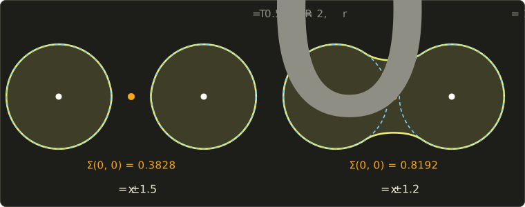
The yellow curves were computed with the marching squares code above, run on a fine grid of field values; the dashed circles are the single-ball surfaces.
That's the whole charm of metaballs: the blend appears automatically, and moving the centers changes the topology (one blob or two) without any special handling, which is great for liquids, clay-like characters and cells.
CSG with min and max
The Boolean operations of CSG (chapter 7) become one-liners for implicit functions with the "negative inside" convention:
A point is in the union if it's inside either shape (the smaller value is negative), in the intersection if it's inside both (the larger value is negative), and in the difference if it's inside A and outside B.
Worked example. Sphere A of radius 3 at the origin and sphere B of radius 2 at , written as distances: and .
| Point | union | intersection | A − B | ||
|---|---|---|---|---|---|
| −3 | 2 | −3 (inside) | 2 (outside) | −2 (inside) | |
| −0.5 | −0.5 | −0.5 (inside) | −0.5 (inside) | 0.5 (outside) | |
| 2 | −1 | −1 (inside) | 2 (outside) | 2 (outside) |
The point lies in both spheres, so it's carved away by the difference.
In a shader the same thing is a few lines:
float sdSphere(float3 p, float3 center, float radius) {
  return length(p - center) - radius;
}

float csgUnion(float a, float b) { return min(a, b); }
float csgIntersect(float a, float b) { return max(a, b); }
float csgSubtract(float a, float b) { return max(a, -b); }
float sdSphere(vec3 p, vec3 center, float radius) {
return length(p - center) - radius;
}
float csgUnion(float a, float b) { return min(a, b); }
float csgIntersect(float a, float b) { return max(a, b); }
float csgSubtract(float a, float b) { return max(a, -b); }float sdSphere(float3 p, float3 center, float radius) {
return length(p - center) - radius;
}
float csgUnion(float a, float b) { return min(a, b); }
float csgIntersect(float a, float b) { return max(a, b); }
float csgSubtract(float a, float b) { return max(a, -b); }The min and max create sharp creases where the shapes meet; replacing them with a "smooth minimum" blends them, metaball-style.
Signed distance functions
The spheres above used a special kind of implicit function: the signed distance function (符号付き距離関数, SDF), whose value is the actual distance to the surface, negative inside.
Its gradient has length 1 (almost) everywhere, and its value tells you how far you can safely step along a ray without crossing the surface, which is the basis of sphere tracing (ray marching).
You've seen 2D distance functions in the GLSL series, chapter 6, and chapter 14 of that series ray-marches 3D scenes built from them; Part 2 of this series treats SDFs properly.
Note that min and max of two SDFs still give the right inside and outside, but the result is only a bound on the distance, not always the exact distance.
9.5 Other shape representations
Some things are hard to model with meshes or patches at all: mountains, coastlines, plants, fire, smoke.
These are usually generated by rules or random processes.
Fractals
A fractal (フラクタル, a word coined by Mandelbrot in 1975) is a shape with detail at every scale, typically self-similar (自己相似性): small parts look like the whole.
The classic example is the Koch curve (コッホ曲線, 1904): start with a segment, cut it into thirds, replace the middle third with two sides of an equilateral triangle, and repeat on every new segment forever.
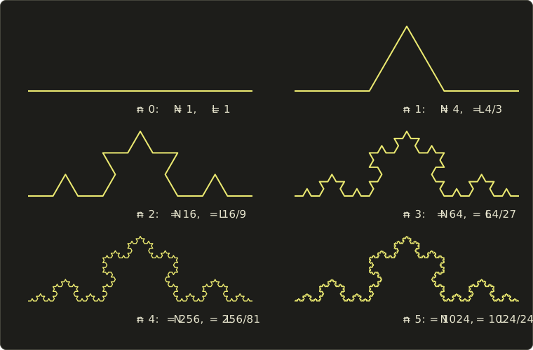
After steps there are segments of length , so the length is , which grows without bound, although the curve stays inside a small region.
How "big" is such a curve? Not 1-dimensional (infinitely long), not 2-dimensional (no area).
The similarity dimension (相似次元, one form of fractal dimension, フラクタル次元) answers it: if a shape consists of copies of itself, each scaled by , then
Check it on ordinary shapes: a segment is 2 copies at scale 1/2, ; a square is 4 copies at scale 1/2, .
The Koch curve is 4 copies at scale 1/3:
Between a line and a plane, as promised.
Real coastlines and mountain profiles behave similarly over a range of scales, which is why fractal methods produce such convincing terrain.
For shapes that aren't exactly self-similar, the dimension is measured by box counting: cover the shape with boxes of size , count how many boxes are needed, and see how the count grows as shrinks.
Midpoint displacement terrain
A practical fractal: midpoint displacement (中点変位法, Fournier, Fussell and Carpenter, 1982).
In 1D: start with a straight line; at each level, move the midpoint of every segment up or down by a random amount, and reduce the random range for the next level (halving it gives a natural-looking roughness; a factor with a parameter controls it).
Worked example. Points , ends , random range , 1, 0.5 at levels 1 to 3, and the "random" numbers listed so you can reproduce it:
| Level | Range | New point = average of neighbors + |
|---|---|---|
| 1 | 2 | |
| 2 | 1 | , |
| 3 | 0.5 | , , , |
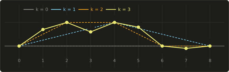
The final profile has big hills from level 1 and small bumps from level 3, the same roughness at every scale.
In 2D the same idea on a grid is the diamond-square algorithm, which creates whole height maps; today terrain is more often made by summing several octaves of a smooth noise function (fractional Brownian motion), which you can try in the GLSL series, chapter 8.
L-systems
An L-system (Lindenmayer system, L-system, 1968), invented by the biologist Aristid Lindenmayer to describe how plants grow, is a string rewriting system: an axiom (the start string) and rules that replace every symbol at the same time, generation after generation.
Worked example 1, no geometry. Axiom A, rules and :
A → AB → ABA → ABAAB → ABAABABA.
The lengths 1, 2, 3, 5, 8 are the Fibonacci numbers, a hint of how compact rules produce growth patterns.
To make a shape, the string is read as commands for a turtle (タートル) that walks on the plane:
| Symbol | Turtle action |
|---|---|
| F | move forward one step, drawing a line |
| + | turn left by the angle |
| − | turn right by |
| [ | remember the current position and heading (push onto a stack) |
| ] | go back to the last remembered state (pop) |
The brackets create branches.
Worked example 2. Axiom F, rule , , step length 1, the turtle starting at the origin heading up (90°).
Generation 1 is the string F[+F]F[−F]F.
The turtle draws F to ; pushes; turns to 120° and draws to ; pops back to heading 90°; draws to ; pushes; turns to 60° and draws to ; pops; draws to .
A stem of three steps with a branch to the left and one to the right.
Each generation replaces every F by 11 symbols, so the number of F's is and the string lengths are 1, 11, 61, 311, 1561 (each F becomes 11 symbols, the other symbols are copied).
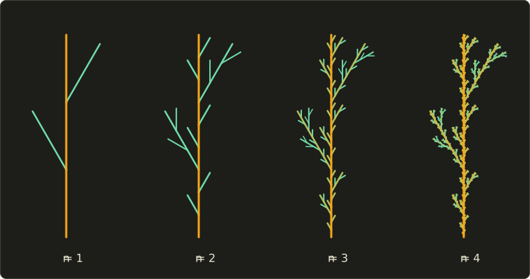
Real plant models add 3D turns (roll and pitch), random choices between rules (stochastic L-systems), parameters for lengths and widths, and leaves and flowers; tools for trees and vegetation in film and games are built on these ideas.
Particle systems
Fire, smoke, explosions, sparks and water spray have no surface at all.
Reeves (1983) modeled them as a particle system (パーティクルシステム), first used for the "Genesis" sequence of the film Star Trek II: The Wrath of Khan (1982): a cloud of many small particles, each with a position, velocity, color, transparency, size and lifetime.
Every frame, new particles are emitted (with random variation around mean values), all particles are moved by their velocity and forces like gravity or wind, their attributes change with age, and particles whose lifetime is over die.
The shape is the statistical result of thousands of simple, random particles; Reeves and Blau (1985) extended the idea to grass and trees, where each particle leaves a trail that becomes a blade or a branch.
A quick count: an emitter that creates 500 particles per second, each living 2 seconds, settles at about particles alive at any moment.
On a GPU, millions of particles are simulated in compute shaders and usually drawn as small camera-facing quads (billboards) with a texture.
Their motion (forces, collisions) belongs to physics-based animation, chapter 14.
Point clouds and point-based rendering
A 3D laser scanner or photogrammetry (below) measures a point cloud (点群): millions of points on a surface, each with a position and often a color and a normal, but with no connectivity.
You can turn it into a mesh (surface reconstruction, for example Poisson surface reconstruction), or render the points directly: point-based rendering draws each point as a small disk or ellipse oriented by its normal, a splat (スプラット), and overlapping splats blend into a closed-looking surface.
Point rendering is natural when there are more points than pixels anyway (huge scans, distant detail), and the recent 3D Gaussian splatting (2023) represents whole scenes as millions of semi-transparent Gaussian splats fitted to photographs.
The scanners themselves are part of chapter 17.
Procedural modeling
Procedural modeling (プロシージャルモデリング, 手続き型モデリング) means writing rules or programs that generate the geometry, instead of placing every vertex by hand.
Fractals, L-systems and particle systems are all examples; others are noise-based terrain, rock and cloud generators, and shape grammars for buildings: a facade is split into floors, floors into windows and walls, by rules with random parameters, and a whole city of different buildings comes from a few pages of rules (the CGA shape grammar behind the CityEngine tool is a well-known example).
The benefits are huge variety from little data and easy changes (change a rule, every building updates); the drawback is that getting exactly the shape an artist has in mind is harder than modeling it directly.
Node-based tools like Houdini, and Blender's Geometry Nodes, are procedural modeling in practice.
Image-based modeling and photogrammetry
Finally, shapes can come from photographs.
Photogrammetry (フォトグラメトリ) takes many photos of an object from different positions, finds matching features between them, recovers the camera positions and a sparse point cloud (structure from motion), then a dense point cloud and a textured mesh (multi-view stereo).
This image-based modeling (イメージベーストモデリング) is how many game and film assets of real places and objects are made today.
Rendering directly from images, without building a model, is image-based rendering in chapter 12, and 3D input devices are in chapter 17.
9.6 Choosing a representation
Every representation is good at something and bad at something else:
| Representation | Stores | Good at | Weak at |
|---|---|---|---|
| polygon mesh | vertices, faces (indices) | drawing on GPUs, any shape, compact with indexing | curved surfaces only approximated, inside test needs a closed mesh |
| subdivision surface | coarse control mesh + rules | smooth surfaces of any topology, easy to edit | must be subdivided (to a mesh) to draw |
| parametric patches (ch. 8) | control points | exact smooth surfaces, CAD precision | complex topology needs many stitched patches |
| voxels | value per grid cell | inside test, CSG, scanned volumes | memory grows with the cube of resolution, blocky |
| octree | adaptive cells | voxel data with less memory, spatial search | more complex access |
| implicit surface | a function | inside test, blending, topology changes | listing surface points, texturing |
| fractal, L-system | rules + random numbers | natural detail from little data | precise control |
| particles | many small points with attributes | fire, smoke, spray | solid surfaces |
| point cloud | measured points | scanned data, huge detail | no connectivity |
In practice they're converted into each other all the time: a CT volume becomes a mesh by marching cubes, a subdivision cage becomes a mesh by subdividing, a point cloud becomes a mesh by reconstruction, and a mesh becomes voxels (voxelization) for physics or global illumination.
Exam points
- An indexed mesh stores each vertex once in a vertex buffer and the triangles as indices; a triangle strip needs indices for triangles.
- Vertex normals are averages of face normals (unweighted, area- or angle-weighted); a hard edge is made by splitting the vertex, not by averaging.
- LOD switches between versions by distance or screen size; the visible jump is popping. Edge collapse removes 1 vertex, 3 edges and 2 triangles.
- Catmull–Clark: any polygons in, quads out; face point, edge point, vertex point ; regular valence 4; generalizes bicubic B-splines. Loop: triangles, each split into 4; regular valence 6. Doo–Sabin: dual scheme, biquadratic. All three are approximating.
- Voxels = spatial occupancy enumeration; memory grows with the cube of the resolution. Octree: split partial cubes into 8.
- Marching cubes: input a scalar volume and an iso value, output triangles; 256 cases, 15 basic patterns, linear interpolation along edges, ambiguous faces can leave holes.
- Implicit surface : the sign gives inside or outside; metaballs sum fields and threshold them; CSG by min and max.
- Fractal (similarity) dimension ; Koch curve .
- L-systems rewrite all symbols in parallel; a turtle interprets the string, brackets make branches. Particle systems (Reeves 1983) model fuzzy phenomena such as fire and smoke.
9.7 Summary
- A polygon surface approximates a curved surface with flat polygons; GPUs draw triangles because they're always flat and convex.
- Indexed meshes (vertex buffer + index buffer) avoid storing shared vertices several times; strips and fans shorten the index list further.
- Vertex normals are averaged from face normals for smooth shading; hard edges, smoothing groups and texture seams split vertices.
- LOD keeps several versions of a model and chooses by projected size; simplification by edge collapse creates them; OBJ, PLY, STL and glTF store meshes for different purposes.
- Subdivision surfaces refine a coarse cage towards a smooth limit: Catmull–Clark (quads), Loop (triangles), Doo–Sabin (dual); extraordinary vertices are only .
- Voxels store values on a 3D grid (memory grows with the cube of the resolution); octrees split only where needed; CT and MRI produce volume data.
- Marching squares and marching cubes extract iso curves and isosurfaces by case tables and linear interpolation; ambiguous cases need a consistent rule.
- Implicit surfaces make inside tests and blending easy: metaballs sum fields, CSG uses min and max, signed distance functions enable ray marching.
- Fractals, midpoint displacement, L-systems, particle systems, point clouds, procedural modeling and photogrammetry generate or capture shapes that are impractical to model by hand.
9.8 Key terms
| English | 日本語 |
|---|---|
| polygon mesh | ポリゴンメッシュ |
| polygon surface | ポリゴン曲面 |
| indexed mesh | インデックス付きメッシュ |
| vertex buffer | 頂点バッファ |
| index buffer | インデックスバッファ |
| triangle strip | トライアングルストリップ |
| triangle fan | トライアングルファン |
| face normal | 面法線 |
| vertex normal | 頂点法線 |
| hard edge | ハードエッジ |
| smoothing group | スムージンググループ |
| level of detail (LOD) | 詳細度(LOD) |
| popping | ポッピング |
| mesh simplification | メッシュの簡略化 |
| edge collapse | エッジ縮約 |
| subdivision surface | 細分割曲面 |
| control mesh (cage) | 制御メッシュ |
| limit surface | 極限曲面 |
| approximating, interpolating scheme | 近似型、補間型 |
| Catmull–Clark subdivision | カトマル・クラーク法 |
| Loop subdivision | ループ法 |
| Doo–Sabin subdivision | ドー・サビン法 |
| valence | 価数 |
| extraordinary vertex | 特異頂点(エクストラオーディナリー頂点) |
| crease | クリース |
| voxel | ボクセル |
| spatial occupancy enumeration | ボクセル表現(空間占有列挙) |
| octree, quadtree | 八分木(オクトツリー)、四分木 |
| isosurface, isoline | 等値面、等値線 |
| iso value | しきい値 |
| marching squares | マーチングスクエア法 |
| marching cubes | マーチングキューブ法 |
| direct volume rendering | ボリュームレンダリング |
| implicit surface | 陰関数曲面 |
| metaball | メタボール |
| signed distance function (SDF) | 符号付き距離関数 |
| fractal | フラクタル |
| self-similarity | 自己相似性 |
| fractal dimension | フラクタル次元 |
| midpoint displacement | 中点変位法 |
| L-system | L-system |
| turtle | タートル |
| particle system | パーティクルシステム |
| point cloud | 点群 |
| splat | スプラット |
| procedural modeling | プロシージャルモデリング(手続き型モデリング) |
| photogrammetry | フォトグラメトリ |
| image-based modeling | イメージベーストモデリング |
9.9 Challenges
- ★ A terrain of 256 × 256 squares is split into triangles. How many vertices and triangles does it have? Compute the memory as a polygon soup and as an indexed mesh with 32-byte vertices. Can the indices be 16-bit? Why or why not?
- ★★ A square pyramid has its apex at and its base corners at (four triangles and one square). Apply one Catmull–Clark step: compute the face point of the triangle with corners , , , then the new position of the apex (valence 4). How many vertices, edges and faces does the subdivided mesh have, and does Euler's formula still hold?
- ★★ Two metaballs with (for ) and threshold lie on the x axis, a distance apart. For which distances is the midpoint between them inside the surface? Then check the point for centers at : is it inside?
- ★★ For the L-system with axiom F, rule and : write generation 1, give the string length and the number of F's for generations 2 and 3, and compute the turtle's three line endpoints after the first F of generation 1 (start at the origin, heading up, step 1).
- ★★★ The Koch snowflake is three Koch curves on the sides of an equilateral triangle. Show that its perimeter grows without bound, while its area converges, and compute the limit of the area as a multiple of the starting triangle's area. (Hint: count how many new small triangles each step adds and sum a geometric series.)
Multiple choice
Q1 ★ Which of the following correctly describes the marching cubes method?
| A | It converts a polygon mesh into a voxel grid by marking the cubes the mesh passes through. |
| B | It always produces exactly 15 triangles per cube, one for each basic pattern. |
| C | It renders a volume without creating any surface, by accumulating color and opacity along each viewing ray. |
| D | It takes a 3D grid of scalar values and an iso value, and generates triangles approximating the isosurface, looking up each cube's 256 possible corner patterns in a table. |
| E | Because every cube is processed independently, the resulting surface can never contain holes. |
Q2 ★ Which of the following statements about subdivision surfaces is correct?
| A | Loop subdivision is designed for triangle meshes, and in a regular region every vertex has valence 6. |
| B | Catmull–Clark subdivision can only be applied to triangle meshes, and it splits each triangle into four triangles. |
| C | In Catmull–Clark subdivision, a vertex with valence 4 is called an extraordinary vertex. |
| D | Doo–Sabin subdivision is an interpolating scheme: all original vertices remain on the limit surface. |
| E | After one Catmull–Clark step, the faces of the original mesh are kept unchanged and only new faces are added. |
Q3 ★★ A curve is constructed by repeatedly replacing every segment with 8 segments, each 1/4 as long. What is the similarity (fractal) dimension of the limit curve?
| A | 2 |
| B | 1.26 |
| C | 1.33 |
| D | 0.5 |
| E | 1.5 |
9.10 Practical assignment
Make a small contour map of an island on graph paper, and along the way use a mesh, normals, marching squares, its ambiguous case and LOD.
You need graph paper (at least 20 × 20 squares, use 4 squares per grid step), a ruler, a pencil, two colored pens and a calculator.
The island is given as heights in meters on a 5 × 5 grid with a spacing of 10 m; goes right, goes up the page, and the height plays the role of the third axis (right-handed: east, north, up).
Negative heights are under water.
Rows are listed from the top () to the bottom ():
| 4 | −6 | −5 | −4 | −3 | −6 |
| 3 | −4 | 4 | −2 | 6 | −3 |
| 2 | −3 | 12 | 20 | −1 | −4 |
| 1 | −5 | 8 | 15 | 3 | −2 |
| 0 | −6 | −4 | −5 | −3 | −6 |
- The mesh. Each grid square becomes two triangles. Count the vertices, triangles and indices, and compute the memory as a polygon soup and as an indexed mesh (32-byte vertices, 16-bit indices).
- A normal. Estimate the vertex normal at the summit with central differences: , likewise for , and . Normalize it and compute how many degrees the slope is tilted from horizontal.
- The coastline. Draw the grid and write each height next to its point. With iso value , mark land and water points, write the case number of each of the 16 cells, and compute every crossing point by linear interpolation (keep three decimals).
- The ambiguous cell. One cell has diagonal land corners. Find it, decide it with the center average, and draw the coastline with the first pen. Then draw, in pencil, what the other choice would have looked like. How many islands do you get with each choice?
- Area. Compute the area enclosed by your coastline with the shoelace formula (the points in order around the loop, the last one followed by the first) and convert it to square meters.
- A second contour. With the second pen, draw the 10 m contour line the same way.
- A coarser LOD. Keep only every other sample (the 3 × 3 grid at ) and draw the coastline of this coarse version. Compare its shape and area with step 5: which details disappeared?
How to check yourself: every crossing point lies between its two grid points, on the side of the one whose height is closer to the iso value; the coastline from step 4 is a single closed loop with 16 points; the 10 m contour lies completely inside the coastline; the normal of step 2 has length 1 and leans towards the side where the ground falls away (its and parts are positive, because the ground drops towards and ); and the coarse coastline encloses a smaller area than the fine one.
コメント(0)
まだコメントはありません。
ログインするとコメント出来ます。