27. HDR and Advanced Image Processing
Chapter 15 taught the image processing of the exam syllabus: histograms, tone curves, convolution, the bilateral filter, pyramids, and one global tone mapping operator, Reinhard's .
It ended with a promise: "local operators adapt to each region like the eye does (Part 2)".
Chapter 16 merged bracketed photos into HDR images, showed why deconvolution is fragile, and used a joint bilateral filter for flash/no-flash photography.
This chapter keeps the promise and goes further.
We'll follow light from the renderer to the screen: scene-referred and display-referred values, exposure with real camera numbers, the filmic curves games use, local tone mapping, and the HDR transfer functions PQ and HLG.
Then we'll open the toolbox of advanced filtering (the FFT and the convolution theorem, Wiener deconvolution, the bilateral grid, the guided filter, non-local means) and end with optical flow, JPEG's DCT and the block formats GPUs read directly.
This is Part 2 and goes beyond the syllabus, but almost everything here deepens a syllabus item of chapter 15: per-pixel tone and color conversion (画素ごとの濃淡変換と色変換) and region-based conversion (spatial filtering) (領域に基づく画像変換(空間フィルタリング)), plus the color spaces and gamma of chapter 3 and the compression of chapter 2; the exam points say where.
Learned upscalers and neural denoisers belong to chapter 29.
All test images are procedural, and all results were computed with the text's formulas.
27.1 The HDR pipeline end to end
Scene-referred and display-referred
A renderer computes radiance, and a camera sensor counts photons: both produce numbers proportional to the light in the scene.
The sun can be a million times brighter than a shadow, so these numbers go from 0 to "anything".
Values like that are scene-referred (シーン参照): they describe the scene, not any screen.
A screen can only show light from black up to its peak: an ordinary monitor about 100 to 300 cd/m² (the unit of luminance of section 22.1, also called the nit), an HDR television 1,000 cd/m² or more at the time of writing.
Values that say what the display should emit are display-referred (ディスプレイ参照).
Everything in between is the display transform: the part of the pipeline that decides how a scene with a dynamic range of 17 stops is shown on a device with 10.
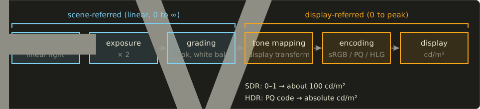
The stages, in order:
- Linear scene light from the renderer (floating-point framebuffer) or camera (RAW, or an HDR merge as in section 16.2).
- Exposure: one multiplication for all pixels; it chooses which part of the scene's range lands mid-display.
- Grading: color correction and the artistic "look", still on scene values.
- Tone mapping: the curve or operator that compresses the range; here scene-referred becomes display-referred.
- Encoding: the sRGB curve of section 3.7 for SDR, PQ or HLG for HDR (section 27.4); the display decodes it back into light.
Exposure never compresses anything, it only slides the scene along the curve; tone mapping is where information is given up.
Exposure in stops
Section 2.3 defined the exposure value (露出値) from the f-number and the shutter time , and chapter 15 used exposure as a multiplication by .
A physically based renderer joins the two, so that artists can light a scene in real units (lux and candela) and "photograph" it with real camera settings.
First the sensitivity (the ISO value) is folded in, giving the exposure value at ISO 100:
Then we need the luminance that just fills the sensor.
ISO 12232's saturation-based sensitivity says the sensor saturates at a focal-plane exposure of lux-seconds, and a lens focused at infinity turns scene luminance into focal-plane exposure with .
Setting them equal gives the largest luminance the camera records:
because .
The exposure step of the renderer is then simply , and means "just saturated".
This is the convention of Lagarde and de Rousiers' physically based Frostbite course notes (SIGGRAPH 2014), and several engines follow it.
Worked example: an evening room.
f/2.8, 1/60 s, ISO 800: and , so .
cd/m².
A wall at 20 cd/m² gets , a lampshade at 300 cd/m² gets , far above 1, and that's fine: it's the tone curve's job.
Outdoors at f/16, 1/100 s, ISO 100 (the photographers' "sunny 16"), and cd/m², nine stops less sensitive.
Automatic exposure and adaptation
Games usually choose the exposure automatically, like a camera's meter and like the eye.
Section 15.4 gave the method: measure the log-average luminance of the frame (usually from a histogram, ignoring the extreme few percent) and put it at a key value such as 0.18.
Jumping to the new exposure in one frame looks wrong, because the eye adapts gradually.
So the exposure, measured in EV, moves toward its target exponentially:
Worked example.
The player walks into a dark room: the target jumps from −1 to +3 EV.
At 60 frames per second ( s) with a time constant s, each frame closes of the gap: the first frame moves EV.
After one second the remaining gap is EV, so the exposure is at .
It behaves the same at any frame rate, and many games use a shorter for getting brighter, as our eyes adapt to light faster than to darkness.
27.2 Global tone mapping operators
What a good curve does
A tone mapping operator (トーンマッピング演算子) maps the exposed scene value to a display value.
A global one (大域的) is a single curve for the whole image, so it's a per-pixel tone conversion exactly like the tone curves of section 15.3, just with an input range that has no upper end.
Plotted against , as photographers and the figure below do, a good curve has three parts:
- a toe (トウ) at the dark end, where the slope drops so that blacks stay black;
- a straight middle part around middle gray (0.18), whose slope sets the contrast;
- a shoulder (ショルダー) that bends the highlights gradually into the top of the range instead of clipping them.
This S-shape is how photographic film responds to light, which is why such curves are called filmic (フィルミック).
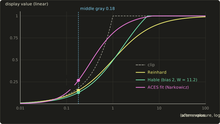
Reinhard's has a shoulder but no toe and a flat middle (images look a little washed out), and it never reaches 1 (the extended version of section 15.4 fixes only that last point, with a white value).
Hable's filmic curve
For the game Uncharted 2, John Hable (2010) published a curve with a toe and a shoulder built from one rational function with six parameters:
with (shoulder strength), , (linear part), (toe strength), and .
His shader multiplies the input by an exposure bias of 2 and divides by the curve's value at the white point , so that becomes exactly 1:
Worked example: middle gray.
: numerator , denominator , so .
For , : numerator , denominator , so .
: a bit darker than Reinhard's 0.153, because of the toe; the curve is steeper above, reaching 0.493 at and 0.918 at .
ACES
The Academy Color Encoding System (ACES) of the Academy of Motion Picture Arts and Sciences is a complete color management framework for film production (section 27.5).
In ACES 1.x the display transform has two steps: the Reference Rendering Transform (RRT), a filmic curve plus color adjustments, and an Output Device Transform (ODT) per display type (sRGB monitor, HDR at 1,000 nits, cinema projector…).
ACES 2.0, released in 2025, replaced them with a redesigned family of output transforms with a gentler tone scale and better gamut mapping.
The full transforms are long, so games often use a fit.
The best known is Krzysztof Narkowicz's (2016), a rational curve fitted to the ACES 1.x RRT + sRGB ODT:
clamped to .
It has a pre-exposure built in (for the original curve, Narkowicz notes, multiply the input by 0.6).
Worked example: , and .
It reaches 1 at (its limit for large is , which the clamp cuts).
It's brighter and more contrasty than Hable's curve, with a stronger toe ( versus 0.0077).
| 0.01 | 0.18 | 0.5 | 1 | 2 | 4 | 16 | |
|---|---|---|---|---|---|---|---|
| Reinhard | 0.0099 | 0.153 | 0.333 | 0.500 | 0.667 | 0.800 | 0.941 |
| Hable | 0.0077 | 0.128 | 0.304 | 0.493 | 0.713 | 0.918 | 1 (clamped) |
| ACES fit | 0.0038 | 0.267 | 0.616 | 0.804 | 0.915 | 0.973 | 1 (clamped) |
Other curves exist, such as AgX, which replaced "Filmic" as Blender's default view in version 4.0; they differ mostly in how they treat saturated highlights.
Per channel or on luminance?
A tone curve maps one number to one number, but a pixel has three.
There are two ways to apply it, and they fail differently.
Worked example. An orange light with linear color :
- Per channel with Reinhard: . The ratio of red to blue was 16, now it's 4: the color is much less saturated, and the brighter the light, the closer it goes to white. Hable per channel gives , the same effect.
- On luminance (section 15.4): , , and the color is scaled by : . The ratios are kept exactly, but red is above 1; clamping it to shifts the hue toward yellow (red to green falls from 4 to 2.6) and loses brightness.
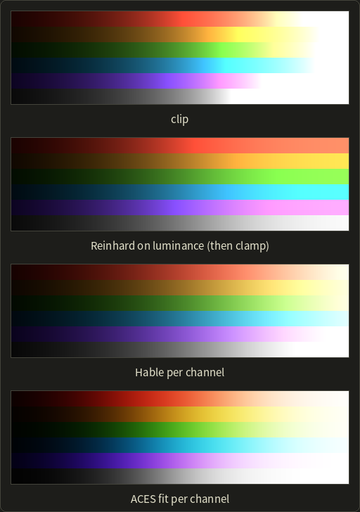
Clipping turns every ramp into flat patches of yellow, cyan, magenta and white; luminance-based Reinhard keeps colors saturated forever (a sun would stay deep orange); the per-channel filmic curves let bright colors desaturate toward white like film does, but shift hues on the way (the blue ramp drifts toward purple, a known complaint about per-channel ACES).
Modern display transforms such as ACES 2.0 and AgX work in a perceptual color space to get this "path to white" without the hue shifts.
In a shader
The tone curve runs in the same full-screen pass as in section 15.4, after the exposure:
// Hable's Uncharted 2 curve, exposure bias 2, white point W = 11.2.
float3 hableRaw(float3 x) {
  const float A = 0.15, B = 0.50, C = 0.10, D = 0.20, E = 0.02, F = 0.30;
  return (x * (A * x + C * B) + D * E) / (x * (A * x + B) + D * F) - E / F;
}

float3 toneMapHable(float3 c) {
  const float W = 11.2;
  return saturate(hableRaw(2.0 * c) / hableRaw(float3(W, W, W)));
}

// Narkowicz's fit of the ACES 1.x RRT + sRGB ODT.
float3 toneMapAcesFit(float3 x) {
  return saturate((x * (2.51 * x + 0.03)) / (x * (2.43 * x + 0.59) + 0.14));
}
// Hable's Uncharted 2 curve, exposure bias 2, white point W = 11.2.
vec3 hableRaw(vec3 x) {
const float A = 0.15, B = 0.50, C = 0.10, D = 0.20, E = 0.02, F = 0.30;
return (x * (A * x + C * B) + D * E) / (x * (A * x + B) + D * F) - E / F;
}
vec3 toneMapHable(vec3 c) {
const float W = 11.2;
return clamp(hableRaw(2.0 * c) / hableRaw(vec3(W)), 0.0, 1.0);
}
// Narkowicz's fit of the ACES 1.x RRT + sRGB ODT.
vec3 toneMapAcesFit(vec3 x) {
return clamp((x * (2.51 * x + 0.03)) / (x * (2.43 * x + 0.59) + 0.14), 0.0, 1.0);
}// Hable's Uncharted 2 curve, exposure bias 2, white point W = 11.2.
float3 hableRaw(float3 x) {
const float A = 0.15, B = 0.50, C = 0.10, D = 0.20, E = 0.02, F = 0.30;
return (x * (A * x + C * B) + D * E) / (x * (A * x + B) + D * F) - E / F;
}
float3 toneMapHable(float3 c) {
const float W = 11.2;
return saturate(hableRaw(2.0 * c) / hableRaw(float3(W, W, W)));
}
// Narkowicz's fit of the ACES 1.x RRT + sRGB ODT.
float3 toneMapAcesFit(float3 x) {
return saturate((x * (2.51 * x + 0.03)) / (x * (2.43 * x + 0.59) + 0.14));
}Both return linear display values; the sRGB encoding follows, by hand or through an sRGB framebuffer, exactly as in the OpenGL series, chapter 21.
Exam points
This ties back to the syllabus item per-pixel tone and color conversion of chapter 15:
- A global operator is a tone curve: equal inputs give equal outputs. Exposure (× ) comes before it, in linear space.
- Filmic curves have a toe, a straight middle part and a shoulder; Reinhard's only has a shoulder and reaches 0.5 at .
- Per channel, a curve desaturates bright colors; on luminance, it keeps the ratios but can push a channel above 1.
27.3 Local tone mapping
What a global curve takes away
A curve that squeezes 17 stops into 10 must lower the contrast somewhere, and a global curve does it everywhere: the texture of a shaded wall loses contrast just because there's a bright window elsewhere.
Our eyes adapt locally instead, and a local tone mapping operator (局所的なトーンマッピング) imitates them: the mapping depends on the neighborhood, so two pixels of the same luminance can come out differently.
Here is the trick, in numbers.
Most of a scene's dynamic range sits in its large-scale brightness changes (room versus window), while the textures we want to see are small ratios on top of them (a brick 1.6 times brighter than the mortar).
Work in of luminance, where ratios become differences, and split each pixel into a base layer (ベース層), the large-scale part, and a detail layer (ディテール層), the rest:
Then compress only the base, and add the detail back unchanged.
The bilateral base: Durand and Dorsey
Frédo Durand and Julie Dorsey ("Fast Bilateral Filtering for the Display of High-Dynamic-Range Images", SIGGRAPH 2002) compute the base with the bilateral filter of section 15.5 on the log luminance, because it smooths the textures but stops at the big edges.
The base is compressed by a factor chosen so that its whole range becomes a target contrast:
Durand's own notes use the target contrast (so ); subtracting puts the brightest base at , display white.
The color is carried along as in section 15.4: each channel is scaled by .
Worked example: one scanline through a window.
Eight pixels, four in the room and four in the window, with a texture that alternates by a factor of :
The scene spans , about 1,260:1.
A bilateral filter with a range (much larger than the 0.2 texture, much smaller than the 2.9 step) averages each side but never across the edge: its base comes out within 0.02 of the side averages, so take in the room and in the window.
The detail is then everywhere.
- Compression: .
- Room: , plus the detail: and , so and .
- Window: plus the detail: and , so and (the brightest texels slightly above 1 clip, or the whole result is scaled down a little).
The room-to-window ratio fell from 794:1 to exactly 5:1, but the texture ratio is still on both sides.
A global curve with the same overall compression (all logs multiplied by 0.241) would have reduced the texture to : barely visible.
Halos
Why not compute the base with an ordinary Gaussian blur?
Because a blur doesn't stop at the edge.
Right next to the window, the blurred base is halfway between the room and the window, so the detail layer there contains a big piece of the edge itself, and since the detail is not compressed, that piece is shown at full strength.
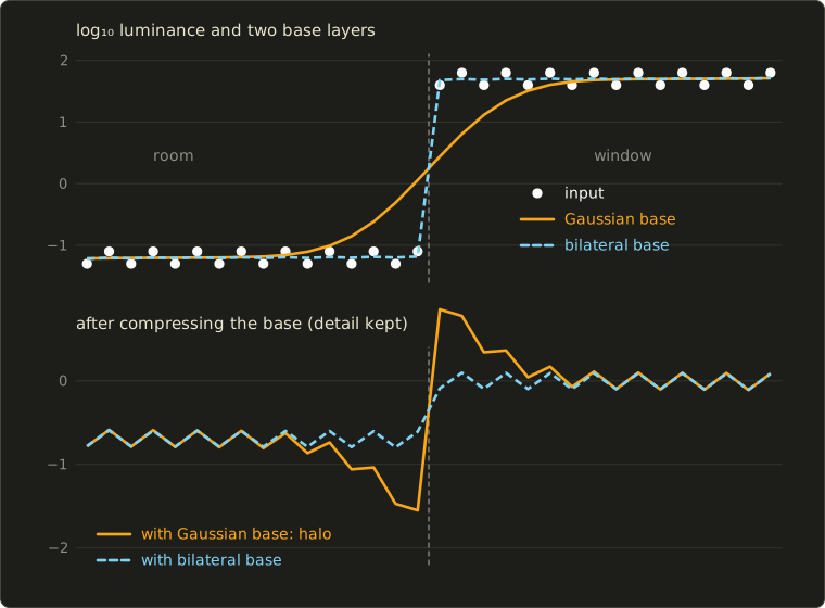
In this longer 32-pixel version of the scanline, a Gaussian with pixels gives the last room pixel a base of instead of , so its detail is instead of , and after compression it comes out 0.94 lower in than with the bilateral base: about 1/9 of the brightness it should have.
That dark band along every bright edge (and the bright band on the other side) is a halo (ハロー), the classic artifact of local tone mapping.
Edge-aware filters (bilateral, guided, the bilateral grid of section 27.7) reduce halos; a smaller target compression hides what remains.
Exposure fusion
There is a way to skip the HDR image entirely.
Tom Mertens, Jan Kautz and Frank Van Reeth's exposure fusion (露出融合, "Exposure Fusion", Pacific Graphics 2007) takes the bracketed LDR photos themselves and blends them directly, choosing for each pixel the photos in which it looks best.
Each photo gets a weight map, the product of three measures:
- contrast: the absolute value of a Laplacian filter on the gray image (section 15.5): edges and texture score high;
- saturation: the standard deviation of R, G and B at the pixel: washed-out pixels score low;
- well-exposedness: how close each channel is to 0.5, , multiplied over the channels.
The weights are normalized to sum to 1 at each pixel.
Worked example: well-exposedness alone.
One gray pixel appears as 0.05, 0.45 and 0.97 in three photos taken 2 stops apart.
The weights are , and , which sum to 1.112, so the normalized weights are 0.072, 0.872 and 0.057.
A per-pixel blend would give .
Blending pixel by pixel makes seams where one photo takes over from another, so the blend is done band by band (section 15.1): each photo becomes a Laplacian pyramid, each weight map a Gaussian pyramid, each level is blended with its own weights, and the result is collapsed.
Coarse levels get smooth weights (no seams), fine levels sharp ones (each detail from the photo where it's best exposed): the multi-band blending of panoramas (section 16.3), used for exposure.
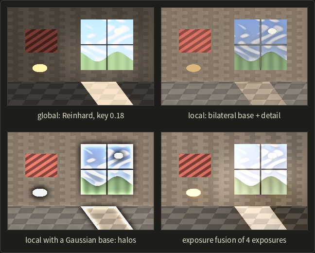
The synthetic room spans 17.2 stops (0.013 to 1,900).
The global curve keeps the room readable but nearly erases the clouds; the bilateral operator shows both, a little flat; the Gaussian base draws halos around the window and the lamp; exposure fusion of four exposures 3 stops apart looks natural without ever building an HDR image.
Local operators in practice
- Reinhard's 2002 paper also has a local version modeled on the photographer's dodging and burning; gradient-domain compression (Fattal and colleagues, 2002) shrinks large log-luminance gradients and re-integrates them with a Poisson solve (section 15.7); local Laplacian filters (Paris, Hasinoff and Kautz, 2011) edit the pyramid directly and avoid halos very well.
- Phone "HDR" photos are local tone mapping of a burst merge (section 16.6).
- Games mostly use a global curve with automatic exposure; at the time of writing, Unreal Engine 5 adds a "local exposure" option with a bilateral base/detail method and an exposure-fusion method.
27.4 HDR displays
Nits, peak and paper white
An SDR signal is relative: 1.0 means "as bright as this display goes", traditionally about 100 cd/m² (sRGB assumes 80).
An HDR display can show highlights ten times brighter, but paper and menus should stay comfortable; only the sun, sparks and speculars should go up.
So HDR production fixes a reference white (基準白), also called paper white: the level of diffuse white.
ITU-R Report BT.2408 recommends 203 cd/m², and Windows lets the user set the level of SDR white, typically around 200 cd/m² on desktop HDR monitors.
From 203 to a 1,000 cd/m² peak there are stops of highlight headroom.
PQ (SMPTE ST 2084)
Stretched to 10,000 cd/m², the sRGB curve would leave visible bands in the darks with 10 bits.
The perceptual quantizer (PQ, 知覚量子化; SMPTE ST 2084, ITU-R BT.2100) was designed from a model of the smallest visible luminance steps (Barten's contrast sensitivity model) so that a 12-bit code step stays below visibility over 0 to 10,000 cd/m², and 10 bits are enough in practice.
Unlike every curve so far, PQ is absolute: a code value means a luminance in cd/m², on every display that can reach it.
The inverse EOTF (from display luminance to the signal ; EOTF, the electro-optical transfer function 電光変換関数, is the display's direction) is
with constants that are exact binary fractions:
| constant | definition | value |
|---|---|---|
| 2610 / 16384 | 0.1593017578125 | |
| 2523 / 4096 × 128 | 78.84375 | |
| 3424 / 4096 = | 0.8359375 | |
| 2413 / 4096 × 32 | 18.8515625 | |
| 2392 / 4096 × 32 | 18.6875 |
and the EOTF itself, which the display applies, is its inverse:
Worked example: 100 cd/m².
and .
Numerator , denominator , ratio 0.991449.
.
So SDR's whole range, 0 to 100 cd/m², uses about half of the PQ signal; the other half is for 100 to 10,000.
The same steps for 1,000 cd/m² give and for 203 cd/m² give 0.5807.
As 10-bit integers, PQ is sent either full range () or, in video, narrow range (, codes 64 to 940, BT.2100):
| luminance (cd/m²) | 0.1 | 80 | 100 | 203 | 1,000 | 10,000 |
|---|---|---|---|---|---|---|
| 0.0623 | 0.4859 | 0.5081 | 0.5807 | 0.7518 | 1.0000 | |
| 10-bit full range | 64 | 497 | 520 | 594 | 769 | 1023 |
| 10-bit narrow range | 119 | 490 | 509 | 573 | 723 | 940 |
A cross-check: Microsoft's Windows HDR documentation gives HDR10 code 497 for white at 80 cd/m², as in the table.
One 10-bit step is about 1% near 100 cd/m² and 9% near 0.01: relative steps, as our eyes need.
HLG (hybrid log-gamma)
HLG (ハイブリッドログガンマ), developed by the BBC and NHK (ARIB STD-B67, 2015, then BT.2100), takes the opposite approach.
It's relative and scene-referred: the camera encodes scene light (normalized so that 1 is the brightest the camera records) with an OETF (opto-electronic transfer function, 光電変換関数, the camera's direction):
with , and .
The square-root lower part resembles what SDR cameras do, so an HLG signal looks acceptable on an old SDR television; the logarithmic upper part packs the highlights, and the constants make the parts meet at , with the same slope.
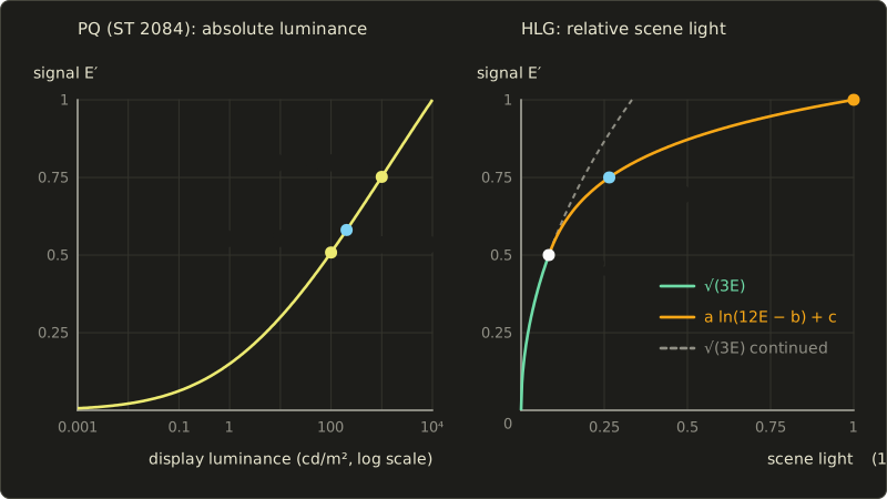
Worked example.
: , and the log branch gives , the same.
: .
The display then applies an OOTF with a system gamma that depends on its peak : per channel ( the scene luminance), .
On a 1,000 cd/m² display ; BT.2408 puts HLG reference white at signal 0.75, which is , and cd/m², the same reference white as PQ.
PQ suits mastered content with metadata, HLG live broadcast that must look right on SDR and HDR sets at once.
Rec.2020 and the HDR10 signal
BT.2100 pairs both curves with the BT.2020 (Rec.2020) primaries of section 3.4.
"HDR10" means PQ, BT.2020 and 10 bits, with static metadata about the mastering display and the content's brightest pixel and frame (MaxCLL, MaxFALL); HDR10+ and Dolby Vision add per-scene metadata.
Converting linear sRGB (BT.709) colors to BT.2020 is a 3 × 3 matrix built from the primaries exactly as in section 3.4:
Each row sums to 1 (white stays white), and pure sRGB red becomes in BT.2020: inside the larger triangle, so all values stay positive.
Rendering for an HDR display
A game with HDR output keeps its renderer and changes the end of the pipeline: it tone maps to the display's peak (from the system or a calibration screen) instead of to 1, puts diffuse white and the UI at the player's paper white (a UI at 1,000 cd/m² is painful), and either encodes BT.2020 with PQ into a 10-bit swapchain or writes linear values to a 16-bit float swapchain.
On Windows the latter is scRGB: sRGB primaries, linear, 1.0 = 80 cd/m², so 1,000 cd/m² is 12.5 and colors outside sRGB have negative components.
The encoder converts the color to BT.2020 with the matrix above, multiplies by the paper white in cd/m², and encodes each channel:
// PQ inverse EOTF (SMPTE ST 2084): luminance in cd/m^2 -> signal 0..1.
float pqEncode(float nits) {
  const float m1 = 2610.0 / 16384.0, m2 = 2523.0 / 4096.0 * 128.0;
  const float c1 = 3424.0 / 4096.0, c2 = 2413.0 / 4096.0 * 32.0, c3 = 2392.0 / 4096.0 * 32.0;
  float p = pow(max(nits, 0.0) / 10000.0, m1);
  return pow((c1 + c2 * p) / (1.0 + c3 * p), m2);
}
// PQ inverse EOTF (SMPTE ST 2084): luminance in cd/m^2 -> signal 0..1.
float pqEncode(float nits) {
const float m1 = 2610.0 / 16384.0, m2 = 2523.0 / 4096.0 * 128.0;
const float c1 = 3424.0 / 4096.0, c2 = 2413.0 / 4096.0 * 32.0, c3 = 2392.0 / 4096.0 * 32.0;
float p = pow(max(nits, 0.0) / 10000.0, m1);
return pow((c1 + c2 * p) / (1.0 + c3 * p), m2);
}// PQ inverse EOTF (SMPTE ST 2084): luminance in cd/m^2 -> signal 0..1.
float pqEncode(float nits) {
const float m1 = 2610.0 / 16384.0, m2 = 2523.0 / 4096.0 * 128.0;
const float c1 = 3424.0 / 4096.0, c2 = 2413.0 / 4096.0 * 32.0, c3 = 2392.0 / 4096.0 * 32.0;
float p = pow(max(nits, 0.0) / 10000.0, m1);
return pow((c1 + c2 * p) / (1.0 + c3 * p), m2);
}27.5 Color management and gamut mapping
ICC profiles
Section 3.4 showed that "RGB" means nothing until we know the primaries, the white and the transfer curve.
Color management (カラーマネジメント) is the bookkeeping that carries this information with every image and converts correctly between devices.
The classic system is the ICC profile (ICCプロファイル) of the International Color Consortium: each device or file has a profile that converts its values to and from a profile connection space (PCS, プロファイル接続空間), CIE XYZ or CIELAB with a D50 white.
Converting from a camera to a printer is then "camera profile into the PCS, printer profile out of it", with profiles instead of converters.
When the printer can't show a color, the profile's rendering intent (レンダリングインテント) decides: perceptual compresses the whole gamut smoothly, relative colorimetric keeps in-gamut colors exact and clips the rest, saturation keeps colors vivid (for charts), and absolute colorimetric also reproduces the paper white (for proofing).
OCIO and ACES
Film and game pipelines use OpenColorIO (OCIO, from Sony Pictures Imageworks, now an Academy Software Foundation project): one configuration file describes every color space of a production and the transforms between them, and every application reads the same file.
The most common configuration is ACES: the archival space ACES2065-1 uses the AP0 primaries, which enclose all visible colors; rendering and compositing happen in linear ACEScg with the AP1 primaries, a little wider than BT.2020; output transforms make the image for each screen.
The working space matters for rendering, because multiplying colors channel by channel gives different results in different primaries.
Gamut mapping
Going from a larger gamut to a smaller one can produce colors that don't exist on the target.
Worked example.
Pure BT.2020 green converted to linear BT.709 with the inverse of the matrix above is : two negative components and one above 1, a color outside the sRGB triangle.
Clipping each channel to gives , sRGB green: its luminance rises from 0.678 to 0.715, and every BT.2020 color beyond sRGB green collapses onto the same point.
Gamut mapping (ガマットマッピング) does better: it moves out-of-gamut colors toward the gray axis at roughly constant hue and lightness, and compresses the colors near the boundary so that neighbors keep their differences, a shoulder for saturation instead of brightness.
Exam points
These ideas extend chapter 3 (color spaces, gamuts, gamma) and the per-pixel conversion item of chapter 15:
- sRGB, DCI-P3 and BT.2020 differ in primaries; converting between linear RGB spaces is a 3 × 3 matrix through XYZ, and the transfer curve is applied outside it.
- SDR signals are relative; PQ is absolute (cd/m², up to 10,000), HLG is relative and scene-referred with a square-root part compatible with SDR.
- Clipping out-of-gamut values changes hue and brightness; gamut mapping compresses toward the gray axis instead.
27.6 The Fourier transform and the FFT
The DFT
Section 15.5 described the frequency domain in words: an image is a sum of waves, smoothing is a low-pass filter, and convolution in space is multiplication in frequency.
Let's do the arithmetic, in 1D first.
The discrete Fourier transform (DFT, 離散フーリエ変換) of samples is
and its inverse is .
With , each is a pair of dot products (linear algebra chapter 4) of the signal with a cosine and a sine of cycles: its magnitude says how much of that frequency there is, its angle (the phase) where the peaks are, and is the plain sum.
Worked example: .
For four samples, , so the factors are just powers of : .
Take :
- ,
- ,
- ,
- .
The values are real because the signal is symmetric; challenge 4 has complex ones.
The convolution theorem, worked
Now blur with the kernel , which is the kernel of chapter 15 centered on sample 0, with the signal wrapping around (circular convolution, ):
- directly: , , , ;
- through frequency: gives , so , and the inverse DFT gives , , , .
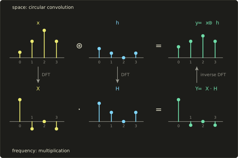
Same answer, and the frequency side explains it: the blur keeps the average (), halves frequency 1, and removes the Nyquist frequency entirely (), just as section 15.5 found for the checkerboard.
That's the convolution theorem (畳み込み定理): , sample by sample.
The DFT treats signals as periodic, so for an ordinary convolution the image and kernel are first zero-padded, or the right edge bleeds into the left.
The FFT
Computed from the definition, the DFT costs multiplications per output, in all.
The fast Fourier transform (FFT, 高速フーリエ変換; Cooley and Tukey, 1965, though Gauss had the idea around 1805) splits the sum into even and odd samples:
and are DFTs of half the length, and , (a butterfly, two outputs from one multiplication).
Repeating the split times leaves butterflies.
Worked example. For our : the even samples have the 2-point DFT , the odd samples have , and with : , , , .
For the FFT needs 5,120 butterflies instead of 1,048,576 multiply-adds: about 200 times less work.
A 2D DFT is separable: transform the rows, then the columns.
Convolving a 1024 × 1024 image with a 64 × 64 kernel directly costs 4,096 multiply-adds per pixel, while FFT, product and inverse FFT of the padded image cost a few hundred; for small kernels direct convolution wins.
Graphics uses it for bloom with large lens-shaped kernels (Unreal Engine offers FFT "convolution bloom" at the time of writing), for ocean height fields (Tessendorf, 2001, an inverse FFT of a wave spectrum every frame), for image alignment by phase correlation, and for deconvolution.
Wiener deconvolution
Section 16.5 showed that undoing a blur is fragile: a blur that has a zero in its frequency response erases that frequency, and dividing by (nearly) zero amplifies the noise without limit.
In frequency, the blurred image is (with the noise), and the naive inverse filter divides by .
The Wiener filter (ウィーナーフィルタ; Norbert Wiener, 1940s) is the linear filter that minimizes the expected squared error; with a noise-to-signal power ratio it's
( is the complex conjugate).
Where the blur keeps the signal strong () it divides by ; where it doesn't, it gives up gracefully.
Worked example: the gain for real with .
| 1 | 0.5 | 0.1 | 0.01 | 0 | |
|---|---|---|---|---|---|
| inverse filter | 1 | 2 | 10 | 100 | ∞ |
| Wiener | 0.99 | 1.92 | 5.00 | 0.99 | 0 |
The largest gain is , at .
For the 3-pixel motion blur of section 16.5, is exactly 0 at : the inverse filter explodes there, the Wiener filter outputs nothing at that frequency, and the error stays bounded.
Richardson–Lucy and learned methods follow the same principle: don't trust frequencies the blur destroyed.
27.7 Edge-aware filtering and denoising
The bilateral filter of section 15.5 smooths without crossing edges, but it's slow (its weights change at every pixel, so it's not a convolution and has no FFT shortcut) and it has artifacts; here are the better tools.
The joint (cross) bilateral filter
The joint bilateral filter (ジョイントバイラテラルフィルタ, also cross bilateral) takes the range weight from a second, guide image and smooths the input :
Flash/no-flash photography (section 16.6) uses the flash photo as the guide; renderers denoise ray-traced shadows and AO with the G-buffer's depth and normals as the guide (chapter 24), and joint bilateral upsampling (Kopf and colleagues, 2007) takes the edges of a half-resolution effect from the full-resolution depth.
The bilateral grid
Jiawen Chen, Sylvain Paris and Frédo Durand (SIGGRAPH 2007) noticed that a bilateral filter is an ordinary Gaussian blur in a higher-dimensional space: lift each pixel to , and pixels on different sides of an edge are far apart in the third dimension.
The bilateral grid (バイラテラルグリッド) is a coarse 3D array over , sampled about once per and once per :
- Splat: add every pixel's value (and a count of 1) into its grid cell.
- Blur: a small Gaussian blur of the grid in all three dimensions.
- Slice: for each pixel, interpolate the grid trilinearly at and divide the value by the count.
Worked example: the size.
A 1920 × 1080 frame with pixels and (on intensities from 0 to 1) gets a grid of cells, 23 times fewer than the 2,073,600 pixels.
Since the blur runs on this small grid, the cost barely depends on (a larger sigma means a coarser grid, not a bigger kernel), and every step is local and GPU-friendly: it made edge-aware filtering of HD video real-time in 2007, and learned camera pipelines that predict a grid of color transforms build on it.
The guided filter
Kaiming He, Jian Sun and Xiaoou Tang ("Guided Image Filtering", ECCV 2010) start from a different idea: inside each small window , the output is a linear function of the guide:
Fitting to the input by least squares, with a penalty that keeps small, gives
and since every pixel lies in many windows, the final output averages their and : .
All the means, variances and covariances are box filters, which cost per pixel with running sums (integral images) whatever the window size: the guided filter is linear-time and exact, not an approximation.
Worked example: self-guided (), , three-pixel windows.
At an edge, : mean 0.4, variance , so and ; the output is , the edge almost unchanged.
In a flat, noisy region, : variance 0.000267, , ; the output is , the noise almost gone.
So plays the role of : variations much smaller than are smoothed, larger ones kept.
Because the output is locally linear in the guide, it avoids the gradient reversal artifacts the bilateral filter can make at strong edges; it's used for haze removal (by the same authors), matte refinement, joint upsampling and real-time denoisers.
Non-local means
Antoni Buades, Bartomeu Coll and Jean-Michel Morel ("A Non-Local Algorithm for Image Denoising", CVPR 2005) asked: why average only with nearby pixels?
Images repeat themselves (bricks, leaves, letters), and a pixel's best partners for averaging are the pixels whose neighborhoods look the same, wherever they are.
Non-local means (非局所平均) gives each candidate pixel in a search window a weight from the difference of the patches around and :
with the mean squared difference of the patches and a filtering strength tied to the noise level.
Worked example (1D, 3-pixel patches, ).
The pixel to denoise is 51, with the patch .
Candidate A has the patch : differences , , weight .
Candidate B, : , weight .
Candidate C is a neighbor of our pixel, : , weight .
With the pixel itself at weight 1: .
A Gaussian blur would have mixed in the 11 of the neighbor and smeared the peak; non-local means averaged it only with other peaks.
The price is time: a 21 × 21 search window and 7 × 7 patches cost about operations per pixel.
BM3D (Dabov and colleagues, 2007) refined the idea; today learned denoisers lead (chapters 23 and 29).
Anisotropic diffusion
Pietro Perona and Jitendra Malik (IEEE PAMI, 1990) saw a Gaussian blur as heat diffusion, , and let less heat flow across strong gradients: anisotropic diffusion (異方性拡散),
With and a step of 0.25 on the row , pixel 1 sees a difference of 10, conductance , and changes by instead of 2.5, while a noise difference of 1 keeps : edges survive, noise melts, over many iterations.
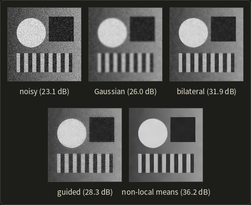
On this test image (noise ) the Gaussian blurs the edges, the bilateral and guided filters keep them (the guided one leaves more noise at these settings), and non-local means wins clearly, because stripes and flat areas offer many identical patches.
The PSNR (ピーク信号対雑音比) is dB; +6 dB halves the RMS error.
27.8 Pyramids, motion and resolution
Laplacian blending revisited
Laplacian pyramid blending (Burt and Adelson, 1983) blends two images with a mask band by band, , using the mask's Gaussian pyramid: at level the transition is about pixels wide, so colors cross over gradually while edges cross within a pixel or two, without seams or ghosts.
Exposure fusion and panorama blending use it.
Optical flow
Video processing (stabilization, frame interpolation, temporal denoising) needs to know where each pixel moves: the optical flow (オプティカルフロー), a vector per pixel.
The basic assumption is brightness constancy: a point keeps its brightness as it moves, .
A first-order Taylor expansion turns this into one linear equation per pixel:
where , are the image gradients (section 15.5) and is the change between the frames.
One equation, two unknowns: a single pixel only tells us the motion along its gradient.
That's the aperture problem (開口問題): through a small hole, a moving straight edge looks the same whatever its motion along the edge.
Lucas–Kanade (Bruce Lucas and Takeo Kanade, "An Iterative Image Registration Technique with an Application to Stereo Vision", IJCAI 1981) assumes that all pixels in a small window move together and solves the equations of the window by least squares, which gives a 2 × 2 system:
Worked example: a window of four pixels.
| pixel | |||
|---|---|---|---|
| 1 | 1 | 0 | −1 |
| 2 | 0 | 1 | −0.5 |
| 3 | 1 | 1 | −1.5 |
| 4 | 2 | 1 | −2.5 |
Sums: , , , , .
The system is , with determinant , so (linear algebra chapter 10) and .
The window moved one pixel right and half a pixel down, and every pixel's equation holds exactly (pixel 4: ).
If all gradients in the window were parallel (a straight edge), the matrix would be singular: the aperture problem again.
Its eigenvalues (here 7.85 and 1.15) say how well the window is constrained; windows where the smaller one is large are good to track (Shi and Tomasi's "good features to track").
The linearization only holds for motions of about a pixel, so implementations iterate and work coarse to fine on a Gaussian pyramid, where a 16-pixel motion at full size is 2 pixels at 1/8 size.
A renderer knows the true motion of every pixel and writes it into a motion vector buffer for temporal anti-aliasing (chapter 20); optical flow still helps with what motion vectors miss (shadows, reflections, particles), for example in frame generation (chapter 29).
Super-resolution
Real-time renderers use the multi-frame super-resolution of section 16.6 on purpose: they jitter the camera by a sub-pixel offset every frame, render at a lower resolution and accumulate the frames along the motion vectors; temporal upscalers add heuristics or a neural network that decide when the history can be trusted (chapter 29).
Exam points
Sections 27.6 to 27.8 deepen the syllabus item region-based conversion (spatial filtering) of chapter 15:
- Convolution in space is multiplication in frequency; smoothing is low-pass. The FFT makes the DFT and pays off for large kernels; the DFT is circular, so pad.
- Deconvolution divides by the blur's frequency response; the Wiener filter limits the gain where the signal is weaker than the noise.
- Edge-preserving smoothing: bilateral (spatial and range weights), joint/cross bilateral (range weight from a guide), guided filter (local linear model), non-local means (patch similarity), anisotropic diffusion (conductance falls at strong gradients). The median filter of chapter 15 is another edge-preserving filter.
- Pyramids: Gaussian (smaller copies), Laplacian (bands, exact reconstruction); blending band by band avoids seams.
27.9 Image compression in depth
The DCT
Section 2.10 listed the steps of JPEG: YCbCr, chroma subsampling, the DCT (discrete cosine transform, 離散コサイン変換) of 8 × 8 blocks, quantization, and lossless coding.
The DCT is a relative of the DFT that uses only cosines and assumes the block is mirrored at its ends instead of repeated, so there's no jump at the block border and the energy of smooth blocks gathers in very few coefficients.
These are its eight 1D basis patterns ( for ); the 64 patterns of section 2.10 are products of a horizontal and a vertical one:
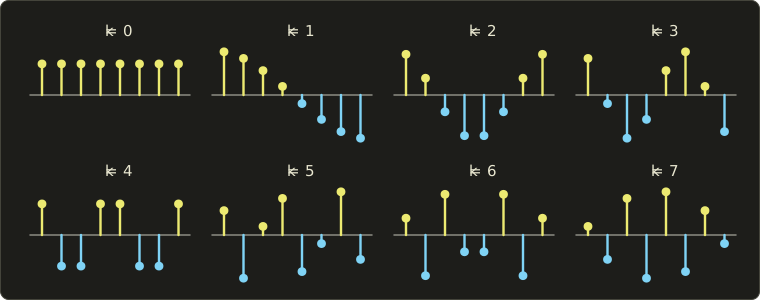
JPEG's forward transform of a block , after subtracting 128 from 8-bit values (the "level shift"), is
with and otherwise.
To work it by hand, take a block whose eight rows are all the same row .
Then the sum of the cosine (which is 1) gives 8, all coefficients vanish, and only the top row of coefficients is left:
Worked example: a smooth row.
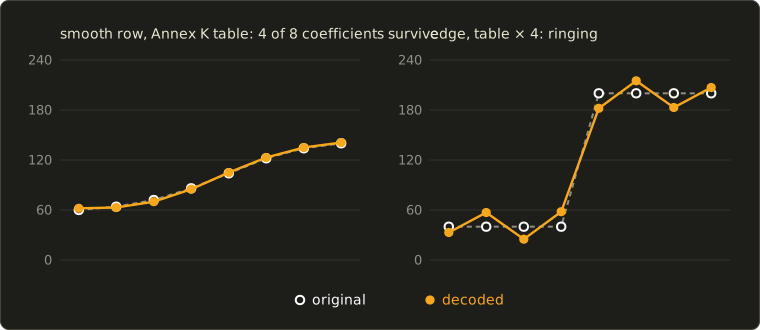
The row 60, 64, 72, 86, 104, 122, 134, 140 (a soft ramp), level-shifted: −68, −64, −56, −42, −24, −6, 6, 12.
, simply the sum.
For the cosines are (positive for the first four samples, negative for the last four), and the weighted sum is , so .
All eight coefficients: −242, −237.5, 15.2, 8.7, −2.0, −0.7, 0.2, −0.9.
Almost all the energy (99.7%) is in the first two.
Quantization
JPEG divides each coefficient by a step from a quantization table (量子化テーブル) and rounds; the rounding is where information is lost.
The JPEG standard's Annex K gives an example luminance table, derived from visibility experiments; its top row (used for ) is 16, 11, 10, 16, 24, 40, 51, 61, so high frequencies get coarser steps.
Encoders scale the whole table for a "quality" setting.
| 0 | 1 | 2 | 3 | 4 | 5 | 6 | 7 | |
|---|---|---|---|---|---|---|---|---|
| −242.0 | −237.5 | 15.2 | 8.7 | −2.0 | −0.7 | 0.2 | −0.9 | |
| step | 16 | 11 | 10 | 16 | 24 | 40 | 51 | 61 |
| level | −15 | −22 | 2 | 1 | 0 | 0 | 0 | 0 |
| decoded | −240 | −242 | 20 | 16 | 0 | 0 | 0 | 0 |
Only four levels are nonzero, and the trailing zeros cost almost nothing after the lossless stage (zigzag order, run-length and Huffman coding).
The decoder multiplies back and applies the inverse DCT: 62, 63, 70, 85, 105, 123, 135, 141.
Every pixel is within 2 of the original; the MSE is 1.75, so the PSNR is dB, invisible.
Ringing and block artifacts
A sharp edge needs high frequencies.
The row 40, 40, 40, 40, 200, 200, 200, 200 has large odd coefficients up to (−64, −579.9, 0, 203.6, 0, −136.1, 0, 115.4).
With the table multiplied by 4 (a low quality setting), the level rounds to 0 and the others get coarse, and the decoded row is 33, 57, 25, 58, 182, 215, 183, 207: ripples on both sides of the edge, overshooting to 215 and undershooting to 25.
That's ringing (リンギング), the "mosquito noise" of section 2.10, the same Gibbs phenomenon as the ideal low-pass filter of section 15.5.
The other classic artifact comes from the blocks themselves.
Each 8 × 8 block is quantized on its own, so at low quality a smooth gradient becomes a staircase of nearly flat blocks whose levels don't match at the borders: block artifacts (ブロックノイズ).
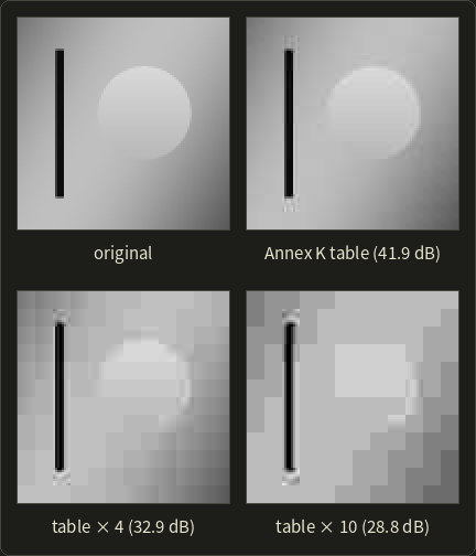
Video codecs (H.264, HEVC, AV1) run a deblocking filter in the coding loop that smooths across block borders only where the step is small enough to be an artifact, an edge-aware filter, and predict blocks from neighbors and other frames; WebP, AVIF and JPEG XL refine the same ingredients and, at the time of writing, AVIF and JPEG XL can store HDR images with PQ or HLG.
Exam points
This extends the image file formats and compression of chapter 2:
- JPEG: YCbCr and chroma subsampling, 8 × 8 DCT, quantization (the lossy step; coarser for high frequencies), zigzag order, run-length and Huffman coding (lossless).
- Smooth blocks concentrate their energy in low frequencies; quantization causes block artifacts (blocks quantized independently) and ringing near edges (high frequencies removed).
- PSNR dB for 8-bit images.
27.10 Texture compression
Different requirements
A texture is read in random order, a few texels at a time (chapter 11), and must stay compressed in memory to save bandwidth.
So texture compression (テクスチャ圧縮) uses fixed-rate block formats: every 4 × 4 block (usually) gets the same number of bits, so any texel's address is a simple calculation, and the texture unit decodes blocks in hardware; encoding can be slow, decoding must be trivial.
BC1 worked
BC1 (also DXT1 or S3TC, from S3 Graphics in the late 1990s) stores a 4 × 4 block of RGB texels in 64 bits:
- two endpoint colors and , each 16 bits in RGB565 (5 bits red, 6 green, 5 blue), 32 bits together;
- 16 indices of 2 bits each (32 bits), one per texel, choosing from a palette of four colors: , , and .
That's 4 bits per texel instead of 24: 6:1 against RGB8, 8:1 against RGBA8.
If as 16-bit numbers, the block switches to a second mode: three colors (, and their average) plus transparent black, for cut-out textures.
The palette lies on a line through RGB space, so BC1 works when a block's colors lie close to one line, which is surprisingly often.
Worked example.
The block is a gradient from amber to blue in four exact steps, plus one red-orange outlier in the top-right corner.
- Endpoints: the two most different colors are amber and blue. In RGB565: , , , so , the 16-bit value = 0xED87. Blue gives = 0x2A93 = 10,899. Since , four-color mode.
- Decode the endpoints to 8 bits by bit replication (, ): , , a few levels off the originals.
- Palette: and .
- Indices: each texel picks the nearest palette entry. The gradient texels match within about 4 levels (the RGB565 rounding). The outlier's distances are 91.6, 213.5, 88.4 and 142.1: it gets index 2, the tan color, an error of 88.
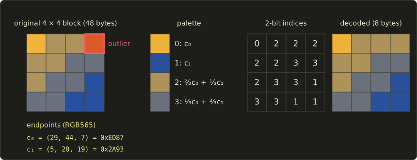
The block shrinks from 48 bytes to 8 and 15 texels are nearly perfect, but the off-line color is lost: the classic BC1 artifact on blocks with two unrelated colors, however hard real encoders search for the endpoints.
The decoder is just this:
#include <cstdint>
#include <cstdio>

struct Rgb { int r, g, b; };

// Expand a 5:6:5 color to 8 bits per channel by bit replication.
Rgb from565(uint16_t c) {
  int r = c >> 11, g = (c >> 5) & 63, b = c & 31;
  return {(r << 3) | (r >> 2), (g << 2) | (g >> 4), (b << 3) | (b >> 2)};
}

// Decode one BC1 block (8 bytes, little endian) into 16 colors, row by row.
void decodeBc1(const uint8_t blk[8], Rgb out[16]) {
  uint16_t c0 = blk[0] | blk[1] << 8, c1 = blk[2] | blk[3] << 8;
  uint32_t idx = blk[4] | blk[5] << 8 | blk[6] << 16 | uint32_t(blk[7]) << 24;
  Rgb p[4] = {from565(c0), from565(c1)};
  if (c0 > c1) {  // four-color mode
    p[2] = {(2 * p[0].r + p[1].r) / 3, (2 * p[0].g + p[1].g) / 3, (2 * p[0].b + p[1].b) / 3};
    p[3] = {(p[0].r + 2 * p[1].r) / 3, (p[0].g + 2 * p[1].g) / 3, (p[0].b + 2 * p[1].b) / 3};
  } else {  // three colors + transparent black
    p[2] = {(p[0].r + p[1].r) / 2, (p[0].g + p[1].g) / 2, (p[0].b + p[1].b) / 2};
    p[3] = {0, 0, 0};
  }
  for (int i = 0; i < 16; ++i) out[i] = p[(idx >> (2 * i)) & 3];
}

int main() {
  const uint8_t blk[8] = {0x87, 0xED, 0x93, 0x2A, 0xA8, 0xFA, 0x7E, 0x5F};
  Rgb px[16];
  decodeBc1(blk, px);
  for (int y = 0; y < 4; ++y) {
    for (int x = 0; x < 4; ++x)
      printf(" (%3d,%3d,%3d)", px[4 * y + x].r, px[4 * y + x].g, px[4 * y + x].b);
    printf("\n");
  }
  return 0;
}
 (239,178, 57) (173,145, 90) (173,145, 90) (173,145, 90)
 (173,145, 90) (173,145, 90) (107,113,123) (107,113,123)
 (173,145, 90) (107,113,123) (107,113,123) ( 41, 81,156)
 (107,113,123) (107,113,123) ( 41, 81,156) ( 41, 81,156)
The index word 0x5F7EFAA8 holds texel 0 in its lowest two bits; the integer division truncates 145.7 to 145 (hardware decoders differ in such rounding by a level).
Addressing: in a BC1 texture 256 texels wide, texel is in block , which is block number at byte offset ; inside it, it's texel , whose index sits at bits and 19 of the index word.
The BCn family, ASTC and ETC2
The desktop formats (Direct3D's names; Vulkan and OpenGL expose the same formats):
| format | content | bits per block | bits per texel | typical use |
|---|---|---|---|---|
| BC1 | RGB (+ 1-bit alpha) | 64 | 4 | opaque color |
| BC3 | RGBA: BC1 color + BC4-style alpha | 128 | 8 | color with smooth alpha |
| BC4 | one channel, two 8-bit endpoints, 3-bit indices | 64 | 4 | roughness, height, masks |
| BC5 | two BC4 channels | 128 | 8 | normal maps (x, y) |
| BC6H | RGB half float | 128 | 8 | HDR (environment maps, lightmaps) |
| BC7 | RGB(A), several modes and partitions | 128 | 8 | high-quality color |
BC7 splits a block into two or three partitions with their own endpoints, which fixes BC1's "one line" limit; BC5 stores a normal map's and and the shader rebuilds (from , : ).
ASTC (Adaptive Scalable Texture Compression, by ARM, presented by Nystad and colleagues at High Performance Graphics 2012 and adopted by Khronos the same year) always uses 128 bits per block but lets the block footprint vary from 4 × 4 to 12 × 12 texels, so the bit rate is : 8 bits per texel at 4 × 4, 3.56 at 6 × 6, 2 at 8 × 8, 0.89 at 12 × 12.
It covers LDR and HDR and one to four channels, and is the common choice on mobile GPUs at the time of writing; ETC2 is required by OpenGL ES 3.0, and supercompressed files (Basis Universal in KTX 2.0) are transcoded at load time to whatever the GPU supports.
Worked example: memory for a 4096 × 4096 texture.
| format | bits per texel | top level | with mipmaps (× 4/3) |
|---|---|---|---|
| RGBA8 | 32 | 64 MiB | 85.3 MiB |
| BC7 | 8 | 16 MiB | 21.3 MiB |
| BC1 | 4 | 8 MiB | 10.7 MiB |
| ASTC 6 × 6 | 3.56 | 7.1 MiB | 9.5 MiB |
| ASTC 8 × 8 | 2 | 4 MiB | 5.3 MiB |
The top level is bytes; the mipmap chain adds a third (section 11.7).
It cuts bandwidth by the same factor, often more important.
27.11 Summary
- Scene-referred linear values are exposed (, ), tone mapped to display-referred values and encoded (sRGB, PQ, HLG); auto exposure adapts exponentially.
- Global operators are tone curves: Reinhard, Hable (0.18 → 0.128), the ACES fit (0.18 → 0.267); per channel they desaturate bright colors, on luminance they keep ratios but overflow.
- Local tone mapping compresses a base layer and keeps the detail; a bilateral base avoids the halos of a Gaussian one. Exposure fusion blends LDR exposures through Laplacian pyramids.
- PQ is absolute (100 cd/m² → 0.508, 1,000 → 0.752), HLG relative and SDR-compatible; reference white is 203 cd/m²; HDR10 = PQ + BT.2020 + 10 bits. ICC, OCIO and ACES carry color spaces; gamut mapping compresses instead of clipping.
- The FFT computes the DFT in ; convolution becomes multiplication; the Wiener filter deconvolves without exploding noise.
- Edge-aware filters: joint bilateral, bilateral grid, guided filter, non-local means, anisotropic diffusion. Lucas–Kanade solves a 2 × 2 system per window.
- JPEG's DCT concentrates smooth blocks; quantization causes ringing and block artifacts. BC1 stores two RGB565 endpoints and 2-bit indices (4 bits per texel); BC7, BC5, BC6H and ASTC (128 bits, 4 × 4 to 12 × 12) cover the rest.
27.12 Key terms
| English | 日本語 |
|---|---|
| scene-referred / display-referred | シーン参照/ディスプレイ参照 |
| exposure value (EV, EV100) | 露出値(EV、EV100) |
| automatic exposure, adaptation | 自動露出、順応 |
| tone mapping operator | トーンマッピング演算子 |
| global / local tone mapping | 大域的/局所的なトーンマッピング |
| toe / shoulder | トウ/ショルダー |
| filmic tone curve | フィルミックなトーンカーブ |
| ACES (RRT, ODT, output transform) | ACES(RRT、ODT、出力変換) |
| base layer / detail layer | ベース層/ディテール層 |
| halo | ハロー |
| exposure fusion | 露出融合 |
| reference white (paper white) | 基準白(ペーパーホワイト) |
| PQ (perceptual quantizer) | PQ(知覚量子化) |
| HLG (hybrid log-gamma) | HLG(ハイブリッドログガンマ) |
| EOTF / OETF / OOTF | 電光変換関数/光電変換関数/光光変換関数 |
| color management | カラーマネジメント |
| ICC profile / profile connection space | ICCプロファイル/プロファイル接続空間 |
| rendering intent | レンダリングインテント |
| gamut mapping | ガマットマッピング(色域マッピング) |
| discrete Fourier transform (DFT) | 離散フーリエ変換(DFT) |
| fast Fourier transform (FFT) | 高速フーリエ変換(FFT) |
| convolution theorem | 畳み込み定理 |
| Wiener filter | ウィーナーフィルタ |
| joint (cross) bilateral filter | ジョイント(クロス)バイラテラルフィルタ |
| bilateral grid | バイラテラルグリッド |
| guided filter | ガイデッドフィルタ |
| non-local means | 非局所平均(ノンローカルミーンズ) |
| anisotropic diffusion | 異方性拡散 |
| PSNR | ピーク信号対雑音比(PSNR) |
| Laplacian pyramid blending | ラプラシアンピラミッドによる合成 |
| optical flow | オプティカルフロー |
| aperture problem | 開口問題 |
| Lucas–Kanade method | ルーカス・カナデ法 |
| super-resolution | 超解像 |
| discrete cosine transform (DCT) | 離散コサイン変換(DCT) |
| quantization table | 量子化テーブル |
| ringing / block artifacts | リンギング/ブロックノイズ |
| texture compression | テクスチャ圧縮 |
| block compression (BC1 to BC7) | ブロック圧縮(BC1〜BC7) |
| ASTC / ETC2 | ASTC/ETC2 |
27.13 Challenges
- ★ Compute the PQ signal and the 10-bit full-range code for 400 cd/m², and the HLG signal for and . Check that your PQ value lies between those for 203 and 1,000 cd/m².
- ★ Compute Reinhard, Hable (with bias 2 and ) and the ACES fit at and . Which curve has the darkest shadows and which keeps the most contrast between 0.09 and 3?
- ★★ A scanline has . Take the side averages as the base, use the target contrast 10, and compute , all eight outputs and the texture ratio. Then compute the texture ratio a global compression of the same strength would leave.
- ★★ Compute the 4-point DFT of (the values are complex this time), multiply by , and invert. Check the result against the circular convolution with computed directly.
- ★★★ Encode a BC1 block of eight pure red and eight pure green texels, then one of red, green and blue. Explain why the second fails, how BC7's partitions fix it, and what a 2048 × 2048 normal map with mipmaps costs in BC5 versus RGBA8.
Multiple choice
Q1 ★ Which of the following statements about tone mapping is correct?
| A | Reinhard's operator maps a scene value of 1 to display white. |
| B | A global tone mapping operator can give two pixels with the same scene luminance different display values when they lie in different regions of the image. |
| C | Applying a tone curve to each RGB channel separately pushes very bright colors toward white, while applying it to luminance and scaling the color keeps the ratios between the channels. |
| D | Exposure is applied after tone mapping, by multiplying the display values by . |
| E | Local tone mapping with a Gaussian-blurred base layer is free of halos, because the Gaussian filter preserves edges. |
Q2 ★ Which of the following statements about HDR video signals is correct?
| A | PQ encodes absolute luminance up to 10,000 cd/m², so a PQ code value means the same luminance on every display that can reach it. |
| B | HLG is display-referred like PQ, and an HLG signal of 1.0 always means 1,000 cd/m². |
| C | The BT.2020 primaries lie inside the sRGB triangle, so converting sRGB colors to BT.2020 produces negative values. |
| D | With PQ, one 10-bit code step changes the luminance by the same number of cd/m² everywhere on the curve. |
| E | Reference white (paper white) should be set to the display's peak luminance so that the user interface looks as bright as possible. |
Q3 ★★ Which of the following statements about filtering and compression is correct?
| A | In JPEG, quantization is lossless and the information is lost in the Huffman coding. |
| B | BC1 stores 16 independent 16-bit colors per 4 × 4 block, so a block takes 32 bytes. |
| C | The cost of the bilateral grid grows with the square of the spatial , because the grid becomes finer. |
| D | ASTC always uses 4 × 4 blocks; only the number of bits per block changes with the quality setting. |
| E | By the convolution theorem, a convolution can be computed by multiplying the DFTs of the zero-padded image and kernel; with the FFT this pays off for large kernels. |
27.14 Practical assignment
One scanline from the scene to the screen and into a file, by hand.
You need a calculator (with , and powers), graph paper and a pencil.
A scanline crosses from a dim room into a sunny window; its scene luminances in cd/m² are 2, 3, 2, 3, 2000, 3000, 2000, 3000.
- Step 1: Exposure. The camera is at f/2.8, 1/60 s, ISO 800. Compute , and the eight exposed values .
- Step 2: Global curves. Apply Reinhard and Hable's curve (bias 2, , clamp at 1) to the eight values, encode them to 8-bit sRGB (section 3.7) and plot both rows on graph paper.
- Step 3: Local tone mapping. Take of the scene values, use the side averages as the base, the target contrast 5, and compute , the eight outputs and the texture ratio on each side. Compare with the global compression of the same strength.
- Step 4: HDR output. On a PQ display, the room's average is shown at 25 cd/m² and the window texels at 600 and 900 cd/m². Compute the PQ signal and the 10-bit full-range code for 25, 203 (paper white), 600 and 900 cd/m².
- Step 5: DCT. A row of a texture in the room reads 50, 70, 50, 70, 50, 70, 50, 70. Compute and for a block made of eight copies of it (the row also has smaller coefficients at ; ignore them here; use the cosines 0.1951, −0.5556, 0.8315, −0.9808, 0.9808, −0.8315, 0.5556, −0.1951), quantize them with the Annex K steps 16 and 61, then quantize again with four times its step. Describe the decoded texture in both cases.
- Step 6: BC1. A gray 4 × 4 block has the rows 40 60 80 100 / 60 80 100 120 / 80 100 120 140 / 100 120 140 160. Pick the endpoints, build the palette (assume first that the endpoints are stored exactly), write the 16 indices, and find the largest error. Then compute the real RGB565 endpoints of 160 and 40 and their 8-bit decoded values.
How to check yourself:
- Step 1: is just below 6, just above 70; room values are hundredths, window values tens.
- Step 2: with Reinhard the four window pixels differ by only one 8-bit level (the window texture is practically gone), and with Hable they are all 255; in the room Hable is darker than Reinhard (the toe).
- Step 3: the base range is exactly 3, is 0.233, the texture ratio stays 1.5 on both sides, and the global version leaves only about 1.1.
- Step 4: 203 cd/m² gives 594 as in the table, and 600 and 900 cd/m² (0.6 stops apart) are more than 40 codes apart.
- Step 5: quantizes exactly (level −34); survives the step 61 as level −1 (stripes of slightly varying contrast come back) and becomes 0 with the step 244, so the row turns into a flat gray of 60: the texture is gone.
- Step 6: the palette is exactly 40, 80, 120, 160, the texels 60, 100 and 140 sit halfway between two entries (largest error 20), and the RGB565 endpoints are no longer pure gray: 160 decodes to (156, 162, 156), a slight green tint.
コメント(0)
まだコメントはありません。
ログインするとコメント出来ます。