20. Anti-Aliasing and Real-Time Transparency
Two problems from Part 1 were left half solved.
In chapter 2 we saw that sampling a scene once per pixel makes jaggies, moiré and crawling edges, and chapter 6 mentioned that GPUs fight them with a cheap trick called MSAA.
In chapter 10 we saw that alpha blending depends on the drawing order, and that sorting transparent objects fails as soon as they intersect.
Both times, the details were postponed to Part 2.
This chapter delivers them.
The first half is anti-aliasing in real time: reconstruction filters, supersampling, MSAA in depth, the post-process methods MLAA, FXAA and SMAA, temporal anti-aliasing (TAA), and specular aliasing.
The second half is transparency in real time: sorting, the under operator, depth peeling, per-pixel linked lists (the A-buffer of chapter 10 on a GPU) and weighted blended order-independent transparency.
All of it goes beyond the exam syllabus, but it deepens two syllabus items: anti-aliasing (chapters 2 and 6) and transparency with alpha blending (chapter 10).
The math is light: weighted averages, the over operator and one projection matrix.
The rasterizer itself (edge functions, the top-left rule, 2×2 quads) is chapter 19; here we only care about where it samples.
20.1 Aliasing in real-time rendering
Section 2.6 gave the rule: with one sample per pixel, an image can hold at most one cycle every 2 pixels, and anything finer comes back disguised as a coarser pattern.
A real-time frame breaks that rule in four different places, each with its own fix:
- Geometric aliasing (幾何学的エイリアシング): triangle edges are hard steps, so silhouettes and intersection lines become staircases, and thin triangles (wires, fences) fall between samples and flicker.
- Shading aliasing (シェーディングのエイリアシング): the fragment shader itself makes detail finer than a pixel, even inside a flat triangle. The classic case is specular aliasing, sparkling highlights on bumpy shiny surfaces (section 20.7).
- Texture aliasing (テクスチャのエイリアシング): minified textures, mostly solved in advance by mipmaps and anisotropic filtering (chapter 11, section 11.7).
- Temporal aliasing (時間方向のエイリアシング): when the camera moves by a fraction of a pixel, the staircases change from frame to frame, so edges crawl and thin details shimmer.
The two honest fixes of section 2.7 still apply: prefilter (as mipmaps do for textures) or take more samples and filter them down.
Prefiltering an arbitrary shader over a pixel is hard, so most of this chapter is about clever ways of taking more samples: per pixel in one frame (SSAA, MSAA) or over several frames (TAA).
Post-process methods are the exception: they guess the missing samples from the finished image.
20.2 Reconstruction filters
When we take several samples per pixel, a filter turns them into one value.
Alvy Ray Smith's well-known 1995 memo "A Pixel Is Not a Little Square" makes the point that a pixel is a point sample, not a square: computing it is a reconstruction (再構成) of the continuous image from the samples, evaluated at the pixel center.
A filter weights each sample by its distance (in pixels) from the center:
Dividing by the sum of the weights keeps a uniform area at its color.
Four filters are common (in 2D they are applied in x and in y):
- Box filter (ボックスフィルタ): for , else 0. Equal weights inside the pixel; what the hardware MSAA resolve does. Its sharp cut-off lets some aliasing through.
- Tent filter (テントフィルタ): . Samples near the center count more, neighbors' samples a little.
- Gaussian filter (ガウシアンフィルタ): ; with it reaches about 1.5 pixels. Very good against aliasing, slightly soft.
- Mitchell–Netravali filter (ミッチェル・ネトラバリフィルタ; Mitchell and Netravali, 1988): a cubic with radius 2 and parameters , ; the recommended balances blur against ringing. Small negative lobes between 1 and 2 pixels sharpen edges slightly.
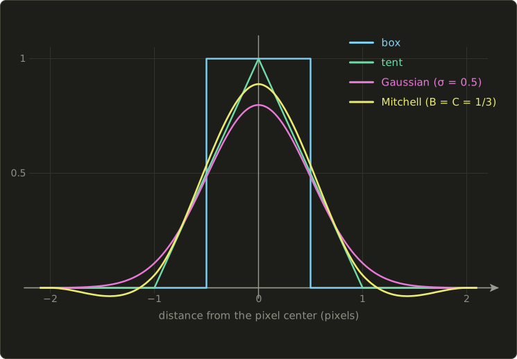
For the Mitchell filter is , and for
With : , , and ; the whole kernel integrates to exactly 1.
The plot scales every filter to an area of 1, which is why the Gaussian peaks at about 0.8 there; constant factors don't matter, because the formula divides by the sum of the weights.
Worked example: box versus tent.
A 1D row has two samples per pixel at from each center; pixel 0 is centered at 0 and pixel 1 at 1, so the samples sit at .
An edge at makes them (white left of it, black right of it).
Box: pixel 0 averages and , giving ; pixel 1 averages and , giving 0.
A hard step, even with two samples per pixel.
Tent: pixel 0 weights the samples at distances 0.75, 0.25, 0.25, 0.75 by 0.25, 0.75, 0.75, 0.25 (sum 2):
The edge position is now visible in the pixel values, and as the edge moves slowly they change smoothly instead of jumping; the price is a little blur.
Offline renderers let you choose the filter; real-time engines mostly use the box filter of the hardware resolve, or let TAA (section 20.6) filter over time.
20.3 Supersampling (SSAA)
Render big, then shrink
Supersampling (スーパーサンプリング, SSAA) from section 2.7 runs the whole pipeline (coverage, depth test and fragment shader) for each of samples per pixel and filters them down.
It fixes geometric, shading and texture aliasing at once, at exactly times the pixel work.
Worked example. 1920×1080 has pixels; 4× SSAA means samples, each with a shader run, a color and a depth.
With 4 bytes of color (RGBA8) and 4 of depth and stencil, that's bytes, about 63.3 MiB, instead of 15.8 MiB.
10 ms of pixel work becomes about 40 ms, so 60 fps is out of reach.
SSAA is used offline, for screenshots, or for old games on new hardware (rendering at 4K for a 1080p screen is SSAA too).
Ordered grid and rotated grid
Where the samples sit matters as much as how many there are.
An ordered grid (格子配置) of 2×2 samples is poor for the edges we notice most, the nearly vertical and nearly horizontal ones.
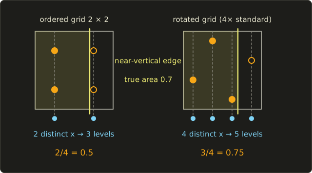
Worked example. A vertical edge at covers 70% of the pixel.
The ordered grid has samples only at and , so a sliding edge can only give (3 levels); here .
A rotated grid (回転格子, RGSS) such as the standard 4× pattern of the next section has , so it steps through 5 levels, and here gives , much closer to 0.7.
In general, samples with all different columns and rows (like non-attacking rooks on a chessboard) give levels for vertical and horizontal edges, while an ordered grid gives only .
That's why GPU sample patterns look scattered rather than gridded.
20.4 Multisample anti-aliasing (MSAA)
The idea
In a typical frame, most aliasing comes from triangle edges, while the shading inside a triangle changes slowly (textures are prefiltered by mipmaps).
Multisample anti-aliasing (マルチサンプルアンチエイリアシング, MSAA) exploits that:
- coverage and depth are tested at sample points per pixel, and each sample stores its own depth, stencil and color;
- the fragment shader runs once per pixel per triangle, and its color is written into every sample the triangle covers and whose depth test passes;
- at the end, a resolve (リゾルブ) averages the sample colors into the final pixel.
A pixel inside a triangle gets identical samples after one shader run.
A pixel on an edge between two triangles runs the shader twice, and the resolve mixes the colors by coverage.
Since depth is stored per sample, the lines where triangles pass through each other are anti-aliased too, as chapter 10 promised.
Sample patterns
Vulkan and Direct3D define standard sample locations (標準サンプル位置) for 2, 4, 8 and 16 samples, supported by almost all desktop GPUs (Vulkan reports it in the limit standardSampleLocations).
In pixel coordinates with the origin at the top-left corner and y down, the 4× pattern is a rotated grid on multiples of :
| Sample | x | y |
|---|---|---|
| 0 | 0.375 | 0.125 |
| 1 | 0.875 | 0.375 |
| 2 | 0.125 | 0.625 |
| 3 | 0.625 | 0.875 |
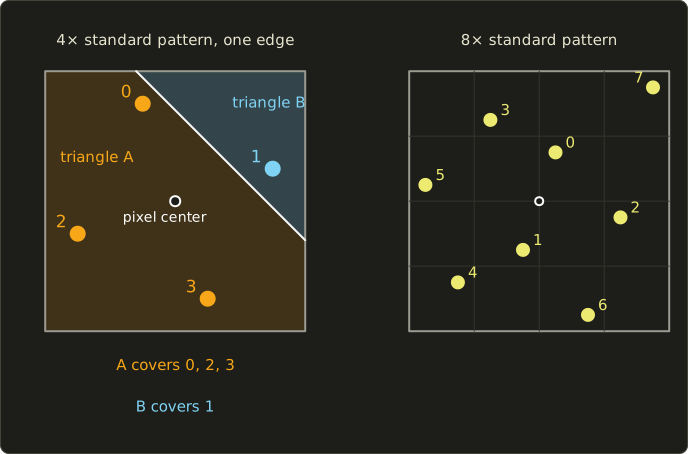
Worked example: one pixel, two triangles
In the picture, the edge is the line , and triangle B is the part where .
- Coverage. is for sample 0, for sample 1, for sample 2 and for sample 3. Only sample 1 exceeds 0.35: B covers sample 1, A covers 0, 2 and 3. As bit masks (bit = sample ): A is , B is .
- Shading. The fragment shader runs twice: A shades to orange , B to blue .
- Writing. Samples 0, 2, 3 receive orange, sample 1 receives blue.
- Resolve. .
B's true share is the triangle , , with area , so the exact color is .
MSAA's estimate of 0.25 is off by 0.04; a single sample at the center would have said 0 and made the pixel pure orange.
Where the shader runs: centroid sampling
B's shader ran once, but at the pixel center , which lies outside B, so its attributes were extrapolated.
A texture coordinate extrapolated past the edge of an atlas region can fetch a neighboring image and leave a colored seam.
Centroid sampling (セントロイドサンプリング) evaluates the attributes at a covered sample (or the centroid of the covered samples) when the center isn't covered: the centroid qualifier in GLSL (centroid in vec2 uv;), the centroid interpolation modifier in Slang and HLSL.
The catch: derivatives (dFdx, ddx) become less accurate, because neighboring pixels may evaluate at different points.
Memory and cost, worked
MSAA saves shading, not memory.
4× MSAA at 1920×1080 still needs the 63.3 MiB of sample buffers of 4× SSAA, plus a single-sample resolve target of bytes (7.9 MiB).
If 8% of the pixels lie on an edge between two triangles, the shader runs about times instead of SSAA's : about 3.7 times less.
GPUs also compress MSAA buffers (a pixel with equal samples is stored as one value plus a flag), which saves bandwidth; tile-based mobile GPUs (chapter 17, section 17.4) keep the samples in on-chip tile memory and write out only the resolved pixels, making 4× MSAA nearly free in bandwidth.
One hidden cost: shaders run in 2×2 pixel quads (chapter 19), and a pixel touched by many tiny triangles runs the shader once per triangle, so dense meshes make MSAA far more expensive than the 8% estimate.
What MSAA does not fix
Shading once per pixel means MSAA does nothing for shading aliasing.
The picture shows a triangle with stripes 1.45 pixels apart, finer than the Nyquist limit of 2 pixels.
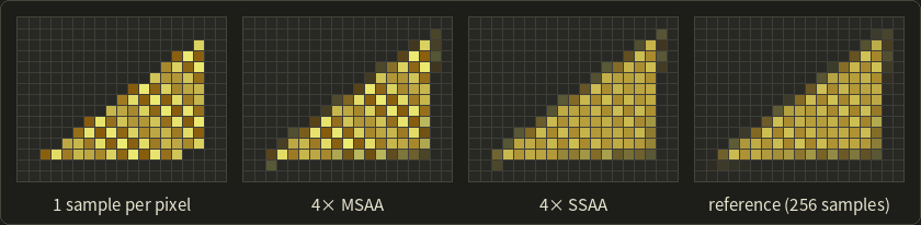
4× MSAA smooths the edges but keeps the same false pattern inside as 1 sample per pixel; 4× SSAA removes most of it.
When that matters, MSAA can switch to sample-rate shading (サンプルシェーディング): sampleShadingEnable and minSampleShading in Vulkan, glMinSampleShading in OpenGL, or simply reading gl_SampleID (GLSL) or SV_SampleIndex (Slang, HLSL) in the shader.
That's SSAA on MSAA hardware, at SSAA's cost.
Alpha-tested geometry is the other hole: leaves and fences drawn as textured quads whose shader discards fragments with alpha below 0.5.
The discard is decided once per pixel, so the leaf's outline stays aliased even with 8× MSAA.
Alpha to coverage
Alpha to coverage (アルファトゥカバレッジ) converts the shader's alpha into a coverage mask: alpha covers about of the samples.
Worked example. With 4× MSAA, gives , so 2 samples are covered and the resolved pixel is half leaf, half background; gives samples, fully opaque.
Along the leaf's edge, where filtered alpha falls from 1 to 0 over a pixel or two, coverage falls smoothly: the edge is anti-aliased, and since the samples write depth like any opaque surface, no sorting is needed.
With 4 samples there are only 5 levels (hardware often dithers the mask to hide them), so it suits the edges of cut-outs, not real glass.
Vulkan enables it with alphaToCoverageEnable, OpenGL with glEnable(GL_SAMPLE_ALPHA_TO_COVERAGE).
CSAA and EQAA
Coverage costs one bit per sample, color and depth much more.
NVIDIA's CSAA (coverage sampling anti-aliasing, GeForce 8800, 2006) and AMD's EQAA (enhanced quality anti-aliasing, Radeon HD 6900, 2010) therefore stored more coverage samples than colors, for example 16 coverage bits but 4 colors, to get gradations close to 16× at a cost close to 4×.
They were driver options rather than API features; the lasting idea is to separate "where is the edge" from "what color is it".
MSAA and deferred shading
Deferred shading (the deferred rendering of chapter 17, section 17.4) breaks MSAA's bargain.
The G-buffer must keep its samples (an edge pixel holds two materials), and the lighting pass must light each sample of edge pixels separately, because averaging normals or materials before lighting is wrong.
Worked example. Chapter 17's G-buffer of 20 bytes per pixel (41.5 MB at 1920×1080) becomes bytes, about 165.9 MB, with 4× MSAA, written and read every frame, and the lighting pass must first find the edge pixels to light them per sample.
Engines did ship this, but the memory and complexity are a big reason why deferred engines moved to post-process and temporal methods, while forward renderers (common in VR) keep MSAA cheap.
In practice
In Vulkan you create images with a sample count such as VK_SAMPLE_COUNT_4_BIT, set rasterizationSamples in the pipeline, and resolve with a resolve attachment or vkCmdResolveImage; in OpenGL you render into a multisample framebuffer and resolve with glBlitFramebuffer, as you'll do in the OpenGL series, chapter 20.
The hardware resolve averages whatever is stored: with linear HDR values, a bright highlight dominates the average, so careful engines tone map per sample or write their own resolve shader.
20.5 Post-process anti-aliasing
The idea
Post-process anti-aliasing works on the finished image with one sample per pixel: it finds staircases, guesses the smooth edge behind them, and blends each edge pixel with its neighbor in the proportion that edge would have covered.
It costs one to three full-screen passes, works with deferred shading and needs no extra samples.
As section 2.7 warned, it can't recover what one sample per pixel already lost: a wire thinner than a pixel stays broken.
MLAA
Morphological anti-aliasing (MLAA, モルフォロジカルアンチエイリアシング; Alexander Reshetov, Intel, 2009) started the family, originally on the CPU:
- Find edges between neighboring pixels whose colors differ by more than a threshold.
- Find shapes: follow the edges and classify each step of the staircase by how its ends turn (the paper's L, Z and U shapes).
- Blend: reconstruct the edge as a line through the middles of the steps, and blend each pixel with the one across the edge by the area the line cuts off.
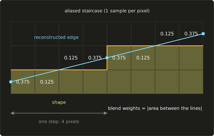
Worked example. The shape's boundary steps up one pixel every 4 pixels.
MLAA joins the middles of the vertical steps, and , so on the first step the edge is , while the aliased boundary sits at height 1.
Each pixel's weight is the area between the two lines over its width:
- pixel 0: . The line is below the boundary, so this shape pixel gets 37.5% of the background color.
- pixel 1: .
- pixel 2: now the line is above the boundary, and the background pixel above gets of the shape's color.
- pixel 3: .
If the true edge really was the line , these are exactly the coverages area sampling (chapter 2's prefilter) would give: MLAA has recovered the anti-aliased edge from a 1-sample image.
When the true edge was a curve or a thin feature, the guess is wrong, and that's where its artifacts come from.
FXAA
FXAA (fast approximate anti-aliasing; Timothy Lottes, NVIDIA; the white paper is dated 2009, and the widely used FXAA 3 and 3.11 were released in 2011) is a single cheap pixel-shader pass that looks only at luma, for example from chapter 3, section 3.6 (it can even use green alone):
- Compute the local contrast of the pixel and its four neighbors (largest minus smallest luma). Below a threshold, leave the pixel alone; most pixels exit here.
- Decide whether the edge is horizontal or vertical, and walk along it in both directions to find where this step of the staircase ends.
- From the pixel's position on the step, compute a sub-pixel offset across the edge and read the image there with bilinear filtering, which blends the pixel with its neighbor in one texture read.
Worked example of the test. Center 0.8, left 0.8, up 0.8, right 0.1, down 0.1: the contrast is far above a typical threshold of about 0.1, so the pixel is processed; a sky with luma between 0.62 and 0.65 has contrast 0.03 and is skipped.
FXAA spread quickly because it drops into any renderer, but it softens fine texture and text, so it must run before the user interface is drawn.
SMAA
SMAA (enhanced subpixel morphological anti-aliasing; Jorge Jimenez, Jose Echevarria, Tiago Sousa and Diego Gutierrez, Eurographics 2012) refines MLAA for GPUs in three passes:
- edge detection on luma, color or depth, with local contrast adaptation (an edge is kept only if it is strong compared to nearby edges, which protects texture detail);
- blending weights: search along each edge for the ends of the step, then look the weights up in a precomputed area texture indexed by the distances and the shape of the ends, with separate handling of diagonals;
- neighborhood blending with those weights.
It keeps corners sharper than MLAA and is more accurate than FXAA, and its variants add 2× MSAA (S2x), a temporal component (T2x) or both (4x) for sub-pixel features.
All three share the same blind spots: sub-pixel features stay broken, motion makes the detected staircases change so edges still shimmer, and texture or text can be mistaken for edges.
The first two are exactly what TAA attacks.
20.6 Temporal anti-aliasing (TAA)
Spreading the samples over time
At 60 fps, consecutive frames are nearly identical.
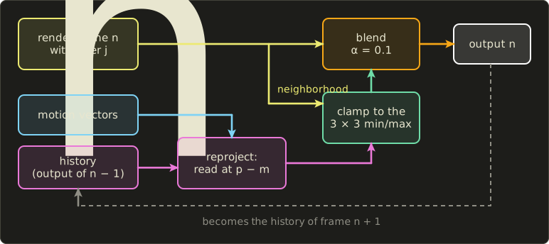
TAA takes one sample per pixel per frame, at a different position inside the pixel each frame, and blends each pixel with its previous values: after 8 frames a still image has effectively 8 samples per pixel at the cost of one.
The idea was published as "amortized supersampling" (Yang, Nehab, Sander, Sitthi-amorn, Lawrence and Hoppe, 2009) and became standard in games through talks such as Brian Karis's "High Quality Temporal Supersampling" (Unreal Engine 4, SIGGRAPH 2014).
It has three parts: jitter, reprojection and history rejection.
Jitter with the Halton sequence
Jitter (ジッタ) shifts the whole projection by a sub-pixel offset that changes every frame.
The offsets should cover the pixel evenly after only a few frames; random offsets clump, but a low-discrepancy sequence (低食い違い量列) spreads out by construction.
The usual choice is the Halton sequence (ハルトン列) with bases 2 and 3.
Its value is the radical inverse of : write in base and mirror the digits behind the point.
Worked example. mirrors to , and mirrors to , so point 6 is .
The first eight points and the jitter in pixels:
| i | i in base 2 | i in base 3 | jitter (pixels) | ||
|---|---|---|---|---|---|
| 1 | 1 | 0.5 | 1 | 0.3333 | (0, −0.1667) |
| 2 | 10 | 0.25 | 2 | 0.6667 | (−0.25, 0.1667) |
| 3 | 11 | 0.75 | 10 | 0.1111 | (0.25, −0.3889) |
| 4 | 100 | 0.125 | 11 | 0.4444 | (−0.375, −0.0556) |
| 5 | 101 | 0.625 | 12 | 0.7778 | (0.125, 0.2778) |
| 6 | 110 | 0.375 | 20 | 0.2222 | (−0.125, −0.2778) |
| 7 | 111 | 0.875 | 21 | 0.5556 | (0.375, 0.0556) |
| 8 | 1000 | 0.0625 | 22 | 0.8889 | (−0.4375, 0.3889) |
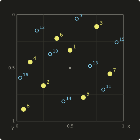
Each new point lands in a large remaining gap, and points 9 to 16 fill the holes between the first eight.
Engines cycle through 8 or 16 of them, skipping index 0, which is the pixel corner .
Low-discrepancy sequences return with Monte Carlo integration in chapter 23.
Jittering the projection. A shift of pixels on a screen pixels wide is in NDC, which spans 2 units.
To add it to after the perspective division, we add to before it, which is exactly what a translation matrix does to a homogeneous vector (Linear Algebra chapter 9):
It works for perspective and orthographic projections alike.
With the linalg series' header, checked by projecting a point:
#include <cstdio>
#include <numbers>
#include "linalg.hh"

// Radical inverse: the i-th point of the Halton sequence in base b.
float halton(int i, int b) {
  float f = 1.0f, r = 0.0f;
  while (i > 0) {
    f /= b;
    r += f * (i % b);
    i /= b;
  }
  return r;
}

// Sub-pixel jitter for frame n (cycle of 8), in pixels, in [-0.5, 0.5).
Vec2 jitter(int frame) {
  int i = frame % 8 + 1;  // skip index 0, which is (0, 0)
  return {halton(i, 2) - 0.5f, halton(i, 3) - 0.5f};
}

// Shift the whole image by j pixels: translate clip space by 2j / size in NDC.
Mat4 jitteredProjection(const Mat4 &proj, Vec2 j, int width, int height) {
  return translate({2.0f * j.x / width, 2.0f * j.y / height, 0.0f}) * proj;
}

// Window coordinates of a view-space point (pixel units, OpenGL convention).
Vec2 toPixels(const Mat4 &proj, Vec3 p, int width, int height) {
  Vec4 c = proj * Vec4{p.x, p.y, p.z, 1.0f};
  return {(c.x / c.w * 0.5f + 0.5f) * width, (c.y / c.w * 0.5f + 0.5f) * height};
}

int main() {
  const int W = 1920, H = 1080;
  Mat4 proj = perspectiveGl(std::numbers::pi_v<float> / 3.0f, float(W) / H, 0.1f, 100.0f);
  Vec3 p{0.0f, 0.0f, -5.0f};  // lands on the image center
  Vec2 base = toPixels(proj, p, W, H);
  printf("unjittered: (%.3f, %.3f)\n", base.x, base.y);
  for (int frame = 0; frame < 8; ++frame) {
    Vec2 j = jitter(frame);
    Vec2 q = toPixels(jitteredProjection(proj, j, W, H), p, W, H);
    printf("frame %d: jitter (%+.3f, %+.3f)  moved by (%+.3f, %+.3f)\n",
           frame, j.x, j.y, q.x - base.x, q.y - base.y);
  }
}
unjittered: (960.000, 540.000)
frame 0: jitter (+0.000, -0.167)  moved by (+0.000, -0.167)
frame 1: jitter (-0.250, +0.167)  moved by (-0.250, +0.167)
frame 2: jitter (+0.250, -0.389)  moved by (+0.250, -0.389)
frame 3: jitter (-0.375, -0.056)  moved by (-0.375, -0.056)
frame 4: jitter (+0.125, +0.278)  moved by (+0.125, +0.278)
frame 5: jitter (-0.125, -0.278)  moved by (-0.125, -0.278)
frame 6: jitter (+0.375, +0.056)  moved by (+0.375, +0.056)
frame 7: jitter (-0.438, +0.389)  moved by (-0.438, +0.389)
The projected point moves by exactly the jitter, and since shifts all of NDC, so does every other point.
With perspectiveVk the code works unchanged, because Vulkan's NDC y and framebuffer y both point down.
Accumulation: an exponential moving average
Instead of storing 8 old frames, TAA keeps one history (履歴) image and updates it with an exponential moving average (指数移動平均):
where is the new jittered frame and is typically around 0.1; frame ends up with weight .
Worked example with :
- the current frame and the four before it weigh 0.1, 0.09, 0.081, 0.0729, 0.0656;
- if each frame's value has noise of variance (an edge pixel flipping in and out as the jitter changes), the average has variance , as good as equally weighted frames;
- after a sudden change, the fraction reached after frames is : 0.41 after 5, 0.65 after 10, 0.90 after 22, about a third of a second at 60 fps.
A smaller is smoother but slower to react, which in motion means ghosting and blur: the central trade-off of TAA.
Reprojection with motion vectors
When things move, the history at pixel shows something else.
So the renderer writes a motion vector (モーションベクトル) per pixel: how far the visible surface moved since the last frame, computed by transforming each vertex with this frame's and the previous frame's matrices (both without jitter) and subtracting the screen positions.
TAA reads the history where the surface was, at : reprojection (再投影, リプロジェクション).
Worked example. At with pixels, the history is read at , between pixel centers, so with a bilinear or bicubic (Catmull–Rom) filter.
That resampling blurs a little every frame and the blur accumulates, which is why TAA looks soft without a sharpening pass.
History rejection: neighborhood clamping
Reprojection fails at disocclusions (ディスオクルージョン, surfaces that were hidden last frame), when lighting or textures change, and for effects without proper motion vectors.
Blending in that wrong history leaves fading trails behind moving objects: ghosting (ゴースト、ゴースティング).
The standard defense is neighborhood clamping (近傍クランプ): the current 3×3 neighborhood says which colors are plausible here now, so the history is clamped to their minimum and maximum before blending.
Worked example (one channel).
The neighborhood holds with center : minimum 0.20, maximum 0.55.
The reprojected history is , left by a bright object that moved away.
Without clamping: , a bright ghost.
Clamped to 0.55: , and the ghost fades quickly.
Variance clipping (Marco Salvi, 2016) is tighter: it uses the neighborhood's mean and standard deviation and clips to ; here , , so with the history is clipped to about 0.414.
Clamping is usually done in YCoCg (luma plus two color differences), where the box fits the colors more tightly than in RGB.
Its cost is flicker: a sub-pixel feature that appears in only some jittered frames changes the range every frame.
The core of a TAA resolve, with the motion vector in UV units:
// One pixel of a TAA resolve. motion is in UV units (this frame minus last frame).
float3 taaResolve(Texture2D<float4> current, Texture2D<float4> history, SamplerState linearClamp,
                  int2 pixel, float2 uv, float2 motion, float alpha) {
  uint w, h;
  current.GetDimensions(w, h);
  int2 size = int2(w, h);
  float3 c = current.Load(int3(pixel, 0)).rgb;
  float3 lo = c;
  float3 hi = c;
  for (int y = -1; y <= 1; ++y) {
    for (int x = -1; x <= 1; ++x) {
      int2 q = clamp(pixel + int2(x, y), int2(0, 0), size - 1);
      float3 n = current.Load(int3(q, 0)).rgb;
      lo = min(lo, n);
      hi = max(hi, n);
    }
  }
  float3 past = history.SampleLevel(linearClamp, uv - motion, 0).rgb;
  past = clamp(past, lo, hi);
  return lerp(past, c, alpha);
}
// One pixel of a TAA resolve. motion is in UV units (this frame minus last frame).
vec3 taaResolve(sampler2D current, sampler2D history, ivec2 pixel, vec2 uv, vec2 motion,
float alpha) {
ivec2 size = textureSize(current, 0);
vec3 c = texelFetch(current, pixel, 0).rgb;
vec3 lo = c;
vec3 hi = c;
for (int y = -1; y <= 1; ++y) {
for (int x = -1; x <= 1; ++x) {
ivec2 q = clamp(pixel + ivec2(x, y), ivec2(0), size - 1);
vec3 n = texelFetch(current, q, 0).rgb;
lo = min(lo, n);
hi = max(hi, n);
}
}
vec3 past = texture(history, uv - motion).rgb;
past = clamp(past, lo, hi);
return mix(past, c, alpha);
}// One pixel of a TAA resolve. motion is in UV units (this frame minus last frame).
float3 taaResolve(Texture2D<float4> current, Texture2D<float4> history, SamplerState linearClamp,
int2 pixel, float2 uv, float2 motion, float alpha) {
uint w, h;
current.GetDimensions(w, h);
int2 size = int2(w, h);
float3 c = current.Load(int3(pixel, 0)).rgb;
float3 lo = c;
float3 hi = c;
for (int y = -1; y <= 1; ++y) {
for (int x = -1; x <= 1; ++x) {
int2 q = clamp(pixel + int2(x, y), int2(0, 0), size - 1);
float3 n = current.Load(int3(q, 0)).rgb;
lo = min(lo, n);
hi = max(hi, n);
}
}
float3 past = history.SampleLevel(linearClamp, uv - motion, 0).rgb;
past = clamp(past, lo, hi);
return lerp(past, c, alpha);
}
lerp(past, c, alpha) and mix(past, c, alpha) both compute ; real implementations add YCoCg, a bicubic history read, a motion-dependent and sharpening.
Strengths, artifacts and upscaling
TAA handles every kind of aliasing (edges, shading, specular, sub-pixel detail) for about one full-screen pass, and it also cleans up effects sampled sparsely per frame, such as screen-space ambient occlusion and ray-traced reflections (chapter 24); modern engines are built around it.
Its typical artifacts are ghosting, blur, flicker on thin features, and smearing of things without motion vectors (particles, scrolling textures).
Once samples are spread over time, the output needn't have the input's resolution: render at a lower resolution with jitter and accumulate into a larger history.
That's temporal upscaling (時間方向アップスケーリング), the principle behind AMD FSR 2 and later, NVIDIA DLSS 2 and later, and Intel XeSS at the time of writing; DLSS, XeSS and FSR 4 replace the hand-written rejection rules partly or fully with a neural network, while FSR 2 and 3 keep hand-written rules; chapter 29 covers them.
20.7 Specular aliasing
A shiny normal-mapped surface defeats all of the above.
Within one pixel the bumps point in many directions, but the shader sees one normal from a mipmap level, so the highlight is either there or not, and it sparkles as the camera moves.
The average of many different normals is a shorter vector; normalized, it describes a smooth mirror with a sharp highlight, while the surface under the pixel is really rough and should have a broad, dim highlight.
Toksvig's method (Michael Toksvig, NVIDIA, 2004) uses that shortness as information.
With the averaged, unnormalized normal, the Blinn–Phong exponent (chapter 10) is reduced by the Toksvig factor
Worked example. Averaging and gives , length 0.8.
With : and , a very wide, dim highlight, as the bumpy surface looks from afar.
Where the normals agree, and nothing changes.
With physically based materials (chapter 22) the same idea is roughness filtering: each mip level's roughness is increased by the variance of the normals it averaged, and some engines also widen it per pixel from the screen-space derivatives of the normal.
The lesson: prefilter the material, not just the texture.
Exam points
Tied to anti-aliasing in chapters 2 and 6:
- Prefiltering (area sampling, mipmaps) removes high frequencies before sampling; postfiltering (supersampling, MSAA, TAA) samples more and filters afterwards.
- SSAA shades every sample. MSAA tests coverage and depth per sample but shades once per pixel per triangle: edges and intersection lines are smoothed, shading and alpha-test aliasing are not.
- Post-process AA works on the finished image (cheap, can't restore sub-pixel detail); TAA accumulates jittered frames with reprojection and history clamping (ghosting and blur are its artifacts).
20.8 Real-time transparency: the problem again
Sorting per object and per triangle
Section 10.12 showed that the over operator, , depends on the order: transparent surfaces must be blended back to front, after the opaque ones, with depth writes off.
The order must be right per pixel, while a GPU draws triangles in the order they arrive.
Engines sort what they can:
- per object: by the distance of each object's center, every frame. Cheap, but wrong for intersecting or cyclically overlapping objects (section 10.2) and for large objects;
- per triangle: for example by keeping index buffers presorted along a few view directions and picking the closest one. Good for one glass object, still wrong where triangles intersect;
- back faces first: drawing a closed object's back faces and then its front faces gives the right order inside convex shapes.
None is exact.
Order-independent transparency (順序非依存の半透明, OIT) means methods whose result doesn't depend on the submission order.
Premultiplied alpha and the under operator
Several OIT methods composite front to back.
With premultiplied alpha (chapter 14, section 14.10), a fragment is stored as , and over simply adds the stored color, : the blend factors (ONE, ONE_MINUS_SRC_ALPHA) on a GPU.
Front to back, keep the accumulated premultiplied color (starting at 0) and the transmittance (透過率) of everything in front (starting at 1):
and finally add the background: .
This is the under operator (アンダー演算).
Worked example with chapter 10's panes, blue in front of red , both , over white: blue gives , ; red gives , ; the background adds for , exactly section 10.12's result for red first, then blue.
Under and over give the same picture from opposite ends of the list, and front to back can stop early once is nearly 0.
The running example
The next sections use one pixel with three fragments, arriving in this order, over a white background:
| Arrival | Color | Distance | |
|---|---|---|---|
| 1 | red (1, 0, 0) | 0.4 | 4 |
| 2 | blue (0, 0, 1) | 0.8 | 6 |
| 3 | green (0, 1, 0) | 0.5 | 3 |
Sorted front to back (green, red, blue) with under:
- green: ,
- red: ,
- blue: ,
- background:
That's the exact answer.
Blending in arrival order with over gives instead: far too blue, because the nearly opaque blue pane at the back was blended over the red one.
20.9 Depth peeling
Depth peeling (デプスピーリング; Cass Everitt, NVIDIA, 2001) finds the per-pixel order with nothing but depth tests, by rendering the transparent geometry several times and "peeling" one layer per pass:
- Pass 1: render with a normal depth test. The depth buffer keeps the nearest transparent surface per pixel: layer 1.
- Pass k: render again with the previous layer's depth in a texture. The shader discards fragments that are not behind the previous layer; among the rest, the ordinary depth test keeps the nearest: layer k.
- After each pass, composite the new layer under the ones before (front to back).
- Stop when a pass produces no fragments (an occlusion query counts them) or after a fixed number of passes.
Opaque geometry is drawn first, and its depth also limits the passes, so nothing hidden behind it is peeled.
Worked example. The running example, with fragments arriving as red, blue, green in every pass:
| Pass | Discard if depth ≤ | Red (4) | Blue (6) | Green (3) | Layer | C after under | T |
|---|---|---|---|---|---|---|---|
| 1 | (nothing) | written (buffer empty) | fails (6 > 4) | wins (3 < 4) | green, 3 | (0, 0.5, 0) | 0.5 |
| 2 | 3 | written | fails (6 > 4) | discarded (3 ≤ 3) | red, 4 | (0.2, 0.5, 0) | 0.3 |
| 3 | 4 | discarded (4 ≤ 4) | written | discarded | blue, 6 | (0.2, 0.5, 0.24) | 0.06 |
| 4 | 6 | discarded | discarded | discarded | none: stop |
Adding the background, : the sorted result, from geometry submitted in the wrong order.
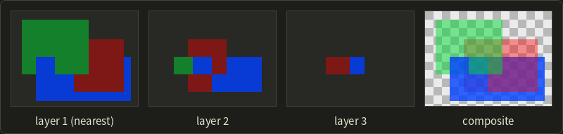
In the picture, the tilted blue quad passes through the other two, so the layer order changes inside each quad; per-object sorting can't get that right, depth peeling gets it right per pixel.
Its cost is the number of passes: 8 transparent layers need 8 full passes over all transparent geometry plus one that finds nothing.
Dual depth peeling (Louis Bavoil and Kevin Myers, NVIDIA, 2008) peels from the front and the back in the same pass with min/max blending of depth, so layers take about passes, 5 instead of 8.
Depth peeling is still used where exactness matters more than speed (CAD, scientific visualization) and as ground truth for faster methods.
20.10 Per-pixel linked lists: the A-buffer on the GPU
The A-buffer of chapter 10, section 10.7 keeps a list of fragments per pixel, then sorts and composites them.
Since about 2010, GPUs can build such lists in a single pass with atomic operations (アトミック操作) in shaders (Jason Yang, Justin Hensley, Holger Grün and Nicolas Thibieroz, "Real-Time Concurrent Linked List Construction on the GPU", 2010).
Three buffers are needed: a head image (one 32-bit index per pixel, cleared to an "end" value every frame), a node pool (one large buffer of nodes with color, depth and the index of the next node) and a counter of the nodes used.
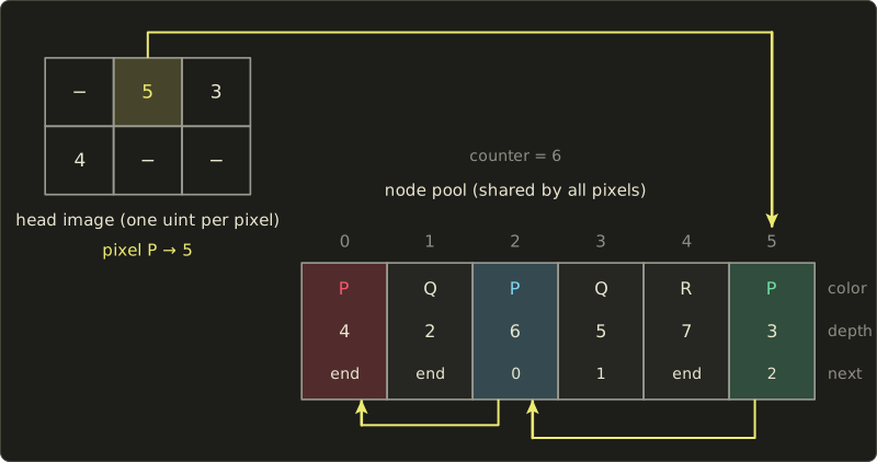
Every transparent fragment, in any order and in parallel with thousands of others:
- allocates a node with
index = atomicAdd(counter, 1), which returns the old value and increments it, so no two fragments get the same index (if the pool is full, the fragment is dropped); - links it in front of its pixel's list with
oldHead = atomicExchange(head[pixel], index); - fills the node: color, depth and
next = oldHead.
The list ends up in reverse arrival order.
In the picture, pixel P's fragments arrived as red, blue, green and got nodes 0, 2 and 5 (other pixels took 1, 3 and 4 in between), so P's list is 5 (green, 3) → 2 (blue, 6) → 0 (red, 4) → end.
Opaque geometry is drawn first, and the transparent shader should use early depth testing (layout(early_fragment_tests) in; in GLSL, [earlydepthstencil] in Slang and HLSL) so hidden fragments never allocate nodes.
struct FragmentNode {
  uint color;   // premultiplied RGBA, 8 bits per channel
  float depth;
  uint next;    // index of the next node, or END
};

static const uint END = 0xFFFFFFFF;

RWTexture2D<uint> heads;                 // cleared to END every frame
RWStructuredBuffer<FragmentNode> nodes;  // the shared node pool
RWStructuredBuffer<uint> counter;        // counter[0] = nodes used, cleared to 0

uint packColor(float4 c) {
  uint4 u = uint4(saturate(c) * 255.0 + 0.5);
  return u.r | (u.g << 8) | (u.b << 16) | (u.a << 24);
}

void insertFragment(uint2 pixel, float4 premul, float depth, uint capacity) {
  uint index;
  InterlockedAdd(counter[0], 1, index);
  if (index >= capacity)
    return;                              // pool full: drop the fragment
  uint oldHead;
  InterlockedExchange(heads[pixel], index, oldHead);
  FragmentNode n;
  n.color = packColor(premul);
  n.depth = depth;
  n.next = oldHead;
  nodes[index] = n;
}
struct FragmentNode {
uint color; // premultiplied RGBA, 8 bits per channel
float depth;
uint next; // index of the next node, or END
};
const uint END = 0xFFFFFFFFu;
layout(set = 0, binding = 0, r32ui) uniform coherent uimage2D heads; // cleared to END
layout(set = 0, binding = 1, std430) buffer Nodes { FragmentNode nodes[]; };
layout(set = 0, binding = 2, std430) buffer Counter { uint counter; }; // cleared to 0
uint packColor(vec4 c) {
uvec4 u = uvec4(clamp(c, 0.0, 1.0) * 255.0 + 0.5);
return u.r | (u.g << 8) | (u.b << 16) | (u.a << 24);
}
void insertFragment(ivec2 pixel, vec4 premul, float depth, uint capacity) {
uint index = atomicAdd(counter, 1u);
if (index >= capacity)
return; // pool full: drop the fragment
uint oldHead = imageAtomicExchange(heads, pixel, index);
nodes[index].color = packColor(premul);
nodes[index].depth = depth;
nodes[index].next = oldHead;
}struct FragmentNode {
uint color; // premultiplied RGBA, 8 bits per channel
float depth;
uint next; // index of the next node, or END
};
static const uint END = 0xFFFFFFFF;
RWTexture2D<uint> heads; // cleared to END every frame
RWStructuredBuffer<FragmentNode> nodes; // the shared node pool
RWStructuredBuffer<uint> counter; // counter[0] = nodes used, cleared to 0
uint packColor(float4 c) {
uint4 u = uint4(saturate(c) * 255.0 + 0.5);
return u.r | (u.g << 8) | (u.b << 16) | (u.a << 24);
}
void insertFragment(uint2 pixel, float4 premul, float depth, uint capacity) {
uint index;
InterlockedAdd(counter[0], 1, index);
if (index >= capacity)
return; // pool full: drop the fragment
uint oldHead;
InterlockedExchange(heads[pixel], index, oldHead);
FragmentNode n;
n.color = packColor(premul);
n.depth = depth;
n.next = oldHead;
nodes[index] = n;
}A full-screen resolve pass then walks each list, copies the nodes into a small local array (say up to 16), sorts them by depth (insertion sort is fastest for such short lists) and composites them over the opaque image: for pixel P, it reads green, blue, red, sorts them to green, red, blue and gets as in section 20.8.
Memory, worked. A node takes bytes.
At 1920×1080 with an average of 4 transparent fragments per pixel, the pool needs nodes, bytes, about 94.9 MiB, plus 7.9 MiB of heads.
The real problem is that the count isn't known in advance: particles in front of the camera can produce 50 fragments per pixel in one frame, and an overflowing pool drops fragments and leaves holes.
Engines allocate for the worst case, grow the pool after an overflow, or keep only the nearest fragments per pixel (k-buffers), which newer hardware features that order a pixel's fragment shader invocations (rasterizer ordered views in Direct3D 12, fragment shader interlock in Vulkan) make practical.
Linked lists are exact as long as nothing is dropped, in one geometry pass.
20.11 Weighted blended order-independent transparency
Giving up on exactness
Exact methods need many passes or unbounded memory.
Weighted blended OIT (重み付きブレンドOIT, WBOIT; Morgan McGuire and Louis Bavoil, Journal of Computer Graphics Techniques, 2013) takes the opposite approach: one pass, two render targets, fixed memory, and an approximation that has no order at all.
In the exact result, two things don't depend on the order: how much of the background is hidden, , and what the background contributes, .
Only the mix of colors inside the covered part does.
WBOIT replaces that mix with a weighted average:
with weights .
Sums and products are commutative, so fixed-function blending accumulates them in any order:
- accumulation target (RGBA16F, cleared to 0, blend
ONE,ONE): each fragment adds ; - revealage target (R8 or R16F, cleared to 1, blend
ZERO,ONE_MINUS_SRC_COLOR): each fragment writes and the blend multiplies the stored value by ; - a full-screen composite divides the sums and blends the average over the opaque image, with the revealage as the background's weight.
The depth test against opaque geometry stays on, depth writes stay off.
With the colors are simply averaged by opacity; the paper's insight is to let fall with distance, so nearer surfaces dominate as they do in reality.
One of its weight functions, for view-space distance , is
tuned for 16-bit float targets and distances from 0.1 to 500; at our distances the and terms are negligible, so .
Worked example
The running example: red at 4, blue at 6, green at 3, over white.
The revealage is , so the layers cover 0.94, exactly as in the sorted result.
With , the average weights the colors by :
The exact answer was : green should dominate because it's in front, but blue does, being the most opaque.
With the depth weight: for green, for red, for blue.
Times (in ) and again (premultiplied color), the shares are green , red and blue , with sum 13.889:
Much closer: the largest error per channel drops from 0.224 to 0.061.
The weights are a heuristic that works when layers are spread out in depth and not too opaque; no weighted average can express "the front layer hides the back layer".
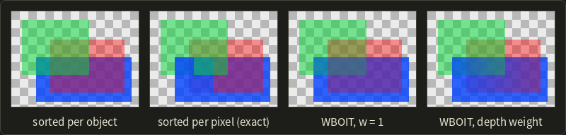
Over the whole picture, the mean error per channel is about 0.018 for per-object sorting, but concentrated in large wrong regions (up to 0.48); 0.029 for and 0.020 for the depth weight, spread thinly (at most 0.32 and 0.22).
WBOIT never pops when objects swap order, and an error that never flickers is usually less visible than a correct image that pops; that's why it's popular for particles, smoke, foliage and glass in games.
struct OitOutput {
  float4 accum : SV_Target0;     // blend ONE, ONE; cleared to 0
  float revealage : SV_Target1;  // blend ZERO, ONE_MINUS_SRC_COLOR; cleared to 1
};

// premul = (alpha * color, alpha); viewDepth = distance from the camera
OitOutput oitAccumulate(float4 premul, float viewDepth) {
  float d = viewDepth / 5.0;
  float w = premul.a * clamp(10.0 / (1e-5 + d * d + pow(viewDepth / 200.0, 6.0)), 1e-2, 3e3);
  OitOutput o;
  o.accum = premul * w;
  o.revealage = premul.a;
  return o;
}layout(location = 0) out vec4 outAccum; // blend ONE, ONE; cleared to 0
layout(location = 1) out float outRevealage; // blend ZERO, ONE_MINUS_SRC_COLOR; cleared to 1
// premul = (alpha * color, alpha); viewDepth = distance from the camera
void oitAccumulate(vec4 premul, float viewDepth) {
float d = viewDepth / 5.0;
float w = premul.a * clamp(10.0 / (1e-5 + d * d + pow(viewDepth / 200.0, 6.0)), 1e-2, 3e3);
outAccum = premul * w;
outRevealage = premul.a;
}struct OitOutput {
float4 accum : SV_Target0; // blend ONE, ONE; cleared to 0
float revealage : SV_Target1; // blend ZERO, ONE_MINUS_SRC_COLOR; cleared to 1
};
// premul = (alpha * color, alpha); viewDepth = distance from the camera
OitOutput oitAccumulate(float4 premul, float viewDepth) {
float d = viewDepth / 5.0;
float w = premul.a * clamp(10.0 / (1e-5 + d * d + pow(viewDepth / 200.0, 6.0)), 1e-2, 3e3);
OitOutput o;
o.accum = premul * w;
o.revealage = premul.a;
return o;
}
The composite pass outputs with alpha equal to the revealage and blend factors (ONE_MINUS_SRC_ALPHA, SRC_ALPHA), which gives ; the two targets need different blend states, which every current API allows.
20.12 Other methods and a comparison
Three more approaches are worth knowing by name:
- Moment-based OIT (Cedrick Münstermann, Stefan Krumpen, Reinhard Klein and Christoph Peters, 2018): a first pass stores a few moments of how absorbance () is distributed over depth in each pixel; a second pass reconstructs from them the transmittance in front of each fragment and composites with it. Fixed memory like WBOIT, but much closer to the sorted result.
- Stochastic transparency (Eric Enderton, Erik Sintorn, Peter Shirley and David Luebke, 2010): treat as the probability that a surface covers each MSAA sample (alpha to coverage with random masks) and use the normal per-sample depth test. Order independent and correct on average, but noisy until enough samples or frames are averaged.
- Ray tracing: hardware ray tracing can find transparent hits in order along each ray and also refract (chapter 12), but is still too costly for heavy particle effects.
| Method | Geometry passes | Memory | Exact? | Typical use |
|---|---|---|---|---|
| Sort per object | 1 | none extra | no (intersections, cycles) | default in most engines |
| Depth peeling | layers + 1 | 2 depth buffers, color | yes | CAD, visualization, reference |
| Dual depth peeling | about layers/2 + 1 | min/max depth, colors | yes | as above, faster |
| Per-pixel linked lists | 1 + resolve | grows with fragments | yes, unless the pool overflows | hair, glass, visualization |
| Weighted blended OIT | 1 + composite | 2 render targets | no (approximate color mix) | particles, smoke, foliage |
| Moment-based OIT | 2 + composite | a few moment targets | no (close) | games, visualization |
| Stochastic transparency | 1 or more, with MSAA | MSAA buffers | on average (noisy) | hair, foliage, with TAA |
Engines mix them: sorting per object by default, OIT for particles and hair, special tricks for a few objects such as a glass of water.
You'll set up blending and sorting yourself in the OpenGL series, chapter 16.
Exam points
Tied to transparency in chapter 10 and compositing in chapter 14:
- Over depends on the order: transparent surfaces go back to front after the opaque ones, depth test on, depth writes off; additive blending is order independent.
- Front to back with under (, ) gives the same result as back to front with over.
- The A-buffer (GPU form: per-pixel linked lists) and depth peeling are exact; weighted blended OIT gets the coverage exactly but only approximates the color mix.
20.13 Summary
- Real-time aliasing comes from geometry, shading, textures (handled by mipmaps) and time. The fixes are prefiltering or more samples plus a reconstruction filter (box, tent, Gaussian, Mitchell–Netravali).
- SSAA shades every sample: everything is fixed at times the cost. Rotated patterns give levels for near-vertical and near-horizontal edges.
- MSAA tests coverage and depth at standard sample positions but shades once per pixel per triangle, then resolves. It smooths edges and intersections, not shading or alpha-test aliasing (sample-rate shading and alpha to coverage help); its memory equals SSAA's, and deferred shading makes it expensive.
- MLAA, FXAA and SMAA find staircases in the finished image and blend along the guessed edge: cheap, but blind to sub-pixel detail and unstable in motion.
- TAA jitters the projection with a Halton sequence, reprojects the history with motion vectors, clamps it to the current neighborhood and blends with an exponential moving average. It handles all aliasing at the price of ghosting and blur, and it underlies temporal upscalers.
- Specular aliasing is fixed by prefiltering the material (Toksvig factor, roughness filtering).
- Transparency needs per-pixel order: sorting is approximate; depth peeling (a pass per layer) and per-pixel linked lists (one pass, unbounded memory) are exact; weighted blended OIT is one pass with fixed memory and an approximate but stable color mix.
20.14 Key terms
| English | 日本語 |
|---|---|
| geometric aliasing | 幾何学的エイリアシング |
| shading aliasing / specular aliasing | シェーディングのエイリアシング/鏡面反射のエイリアシング |
| temporal aliasing | 時間方向のエイリアシング |
| reconstruction filter | 再構成フィルタ |
| box filter / tent filter | ボックスフィルタ/テントフィルタ |
| Gaussian filter | ガウシアンフィルタ |
| Mitchell–Netravali filter | ミッチェル・ネトラバリフィルタ |
| supersampling (SSAA) | スーパーサンプリング |
| ordered grid / rotated grid | 格子配置/回転格子 |
| multisample anti-aliasing (MSAA) | マルチサンプルアンチエイリアシング |
| standard sample locations | 標準サンプル位置 |
| coverage, coverage mask | カバレッジ(被覆率)、カバレッジマスク |
| resolve | リゾルブ |
| centroid sampling | セントロイドサンプリング |
| sample-rate shading | サンプルシェーディング |
| alpha to coverage | アルファトゥカバレッジ |
| post-process anti-aliasing (MLAA, FXAA, SMAA) | ポストプロセスアンチエイリアシング |
| luma, local contrast | ルーマ、局所コントラスト |
| temporal anti-aliasing (TAA) | 時間方向アンチエイリアシング(TAA) |
| jitter | ジッタ |
| Halton sequence, low-discrepancy sequence | ハルトン列、低食い違い量列 |
| exponential moving average | 指数移動平均 |
| history | 履歴 |
| motion vector | モーションベクトル |
| reprojection | 再投影(リプロジェクション) |
| disocclusion | ディスオクルージョン |
| neighborhood clamping, variance clipping | 近傍クランプ、分散クリッピング |
| ghosting | ゴースト(ゴースティング) |
| temporal upscaling | 時間方向アップスケーリング |
| Toksvig factor, roughness filtering | Toksvig係数、ラフネスフィルタリング |
| order-independent transparency (OIT) | 順序非依存の半透明(OIT) |
| under operator | アンダー演算 |
| transmittance | 透過率 |
| depth peeling, dual depth peeling | デプスピーリング、デュアルデプスピーリング |
| per-pixel linked list | ピクセルごとの連結リスト |
| atomic operation | アトミック操作 |
| weighted blended OIT | 重み付きブレンドOIT |
| accumulation, revealage | 蓄積、リビーリッジ(背景の見える割合) |
| moment-based OIT | モーメントベースOIT |
| stochastic transparency | 確率的透明(ストキャスティック透明) |
20.15 Challenges
- ★ A 2560×1440 frame uses 8× MSAA with an RGBA16F color (8 bytes) and a 32-bit depth (4 bytes) per sample. How many bytes, and MiB, do the sample buffers need, and how much does a single-sample RGBA16F resolve target add? How many fragment shader runs would 8× SSAA need per frame?
- ★ Compute the Halton points 9 to 12 (bases 2 and 3) by mirroring digits, their jitter offsets in pixels, and the NDC translations for a 2560×1440 screen. Mark them on the Halton figure and check that they fill gaps between the first eight.
- ★★ A staircase has steps 8 pixels long. Following the MLAA worked example, reconstruct the edge through the middles of the steps and compute the blend weights of the 8 pixels of one step. Check that they are symmetric and that the shape keeps its total area.
- ★★ TAA uses instead of 0.1. Compute the weights of the last four frames, the equivalent number of equally weighted frames, and the frames needed to reach 90% of a new value. Then explain what neighborhood clamping does to a thin wire that is visible in only half of the jittered frames.
- ★★★ Show algebraically that compositing two premultiplied layers front to back with under equals back to front with over. Then show that weighted blended OIT is exact when all layers have the same color, and build a two-layer example (an almost opaque front layer and a differently colored back layer) where it is badly wrong; compute the error for and say how a depth weight changes it.
Multiple choice
Q1 ★ Which of the following statements about MSAA is correct?
| A | MSAA runs the fragment shader once for every sample, so 4× MSAA costs as much shading as 4× SSAA. |
| B | MSAA also removes specular aliasing and other shading aliasing inside triangles. |
| C | With 4× MSAA only the depth buffer grows; the color buffer needs no more memory than without MSAA. |
| D | MSAA works with deferred shading without any extra memory or extra lighting work. |
| E | MSAA tests coverage and depth at several sample points per pixel, but usually runs the fragment shader once per pixel for each triangle that covers it. |
Q2 ★ Which of the following statements about temporal anti-aliasing (TAA) is correct?
| A | TAA renders several samples per pixel in every frame and averages them within that frame. |
| B | TAA shifts the projection by a different sub-pixel offset every frame and blends the current frame with the history, which is reprojected using motion vectors. |
| C | TAA needs no motion vectors as long as only the camera moves. |
| D | Clamping the history to the color range of the current neighborhood is done to give the history more weight and average more frames. |
| E | Unlike post-process methods such as FXAA, TAA can never cause ghosting or blur. |
Q3 ★★ A pixel has two transparent fragments, red and blue , both with , over a black background . What color does weighted blended OIT give with all weights ?
| A | (0.375, 0, 0.375) |
| B | (0.25, 0, 0.5) |
| C | (0.5, 0, 0.25) |
| D | (0.5, 0, 0.5) |
| E | (0.75, 0, 0.75) |
20.16 Practical assignment
Anti-alias and composite one pixel by hand.
You need graph paper, a ruler, colored pencils and a calculator.
You'll follow one pixel through 1-sample rendering, 4× MSAA and eight frames of TAA jitter, then composite a transparent pixel three ways, and compare everything with the exact answer.
The pixel is the unit square with the origin at its top-left corner and y pointing down.
Two triangles meet in it along the line : triangle B is the part above the line (), triangle A the part below.
A is orange and B is blue .
- Draw. Draw the pixel as a 10 cm square, the line from to , and shade B. Mark the pixel center and the four standard 4× sample positions of section 20.4, numbered 0 to 3.
- Exact coverage. Compute B's area (a trapezoid) and the exact area-weighted color of the pixel.
- One sample. Decide which triangle covers the pixel center and write down the color with one sample per pixel.
- 4× MSAA. Test each sample with , write both coverage masks as 4-bit numbers, say how many times the fragment shader runs, compute the resolved color, and say where B's shader is evaluated with and without centroid sampling.
- TAA. Compute the first 8 Halton points (bases 2 and 3) by mirroring digits, plot them in the pixel, count how many lie in B, and average the 8 one-sample results with equal weights.
- Transparency, sorted. Another pixel has three transparent fragments over a black background, arriving as yellow at distance 5, cyan at distance 2 and magenta at distance 3, all with . Composite them back to front with over, front to back with under (write and after each fragment), and in arrival order with over.
- Depth peeling and linked lists. Make a pass table like the one in section 20.9 for the arrival order. Then draw the head and the node pool after the three insertions (nodes 0, 1, 2 in arrival order) and the order in which the resolve reads them.
- WBOIT. Compute the weighted blended OIT result with and compare it with the sorted result. Which part of the formula is exact, and what was lost?
How to check yourself:
- B's area in step 2 is the average of the line's heights at both sides, ; the exact color lies between A and B, closer to A.
- In step 4, the two masks together set all four bits, none twice, and the MSAA color is the average of A and B weighted by sample counts.
- In step 5, the eight x values are all different multiples of , and your estimate of B's coverage is much closer to step 2 than the one-sample result.
- In step 6, over and under agree and the remaining transmittance is ; the arrival-order result differs.
- In step 7, the layers come out nearest first, the pass after the last layer finds nothing, and the list is read in reverse arrival order.
- In step 8, equals from step 6, and the WBOIT color comes out gray, because the three colors are averaged with equal weights.
コメント(0)
まだコメントはありません。
ログインするとコメント出来ます。