24. Real-Time Shadows, Ambient Occlusion and Global Illumination
Chapter 11 gave us shadow maps, bias and PCF, and a first look at ambient occlusion.
Chapter 12 gave us the rendering equation, radiosity, photon mapping and image-based lighting, and ended with a short list of what games do instead.
Both chapters promised more: soft shadows whose penumbra grows the right way, ambient occlusion done properly, and the global illumination tricks that real-time engines actually ship.
This chapter keeps those promises.
Why does this matter?
A game has about 16.7 ms per frame at 60 frames per second, and lighting usually gets only a part of that.
Every technique in this chapter computes a piece of the rendering equation cheaply: the visibility of the light (shadows), the visibility of the "sky" (ambient occlusion), or the light bounced by other surfaces (global illumination), each with its own trade-off between cost, quality and how much of the scene may move.
This is Part 2 material and goes beyond the exam syllabus, but it deepens two of its items: shadowing (影付け, chapter 11) and global illumination (大域照明計算, chapter 12), plus light maps and environment maps from mapping.
We'll use Monte Carlo estimators and importance sampling from chapter 23, and the irradiance and radiance of chapter 12.
24.1 Splitting the problem
Recall the rendering equation of chapter 12, for a point with normal :
Real-time renderers split the incoming light into two parts and treat them with completely different tools:
- Direct light comes straight from the light sources. The integral collapses to a sum over lights, and the only hard part is the visibility of each light: that's shadows (24.2 to 24.4).
- Indirect light has bounced off other surfaces at least once. It arrives from all directions, so it's an integral over the hemisphere: that's global illumination (24.6 to 24.9), and ambient occlusion (24.5) is the cheapest approximation of its visibility part.
A second split runs across the first one: what can be precomputed (baked) and what must be computed every frame.
Baking is cheap at run time and gives beautiful results, but only for things that don't move; much of the history of real-time GI is moving work from the first kind to the second as GPUs got faster.
24.2 Cascaded shadow maps
Section 11.4 ended with the main weakness of shadow mapping for the sun: perspective aliasing.
The shadow map spreads its texels evenly, but the camera sees nearby ground at a much higher density than distant ground, so one map for a 250 m view distance has texels far too large near the camera and pointlessly small far away.
The standard fix is cascaded shadow maps (CSM, カスケードシャドウマップ).
Cut the camera's view frustum along the view direction into slices (cascades, usually 3 or 4), at distances , and give each slice its own shadow map, fitted tightly around that slice.
Near slices are small, so their texels are small; far slices have big texels, but they are far away.
When shading a pixel, the shader picks the cascade whose slice contains the pixel's view depth (and often blends the last few percent of one cascade into the next to hide the seam).
Where to put the splits
Three schemes for the split distances are standard:
The uniform split gives each cascade the same depth range.
The logarithmic split makes every cascade the same ratio of far to near distance, .
The practical split scheme blends the two with a weight between 0 and 1; it was proposed by Zhang and colleagues in 2006 for their parallel-split shadow maps, and Rouslan Dimitrov's NVIDIA whitepaper on cascaded shadow maps (2007) uses it to place the cascades.
Why is the logarithmic split the ideal one?
A rough model makes it clear.
Say the camera has a 90° vertical field of view and an image 1080 pixels tall.
At distance the view is tall, so one pixel covers .
A cascade's 2048 × 2048 shadow map must cover its slice, which at the far end is about wide, so one texel covers about .
The worst place is the near end of the slice, , where texels look largest:
So the quality of a cascade depends only on the ratio , and the logarithmic split makes that ratio the same for every cascade.
Worked example. m, m, cascades.
- Uniform: gives 1, 64.75, 128.5, 192.25, 256.
- Logarithmic: and , so 1, 4, 16, 64, 256.
- Practical with : the averages of the two, , then 72.25, 128.125, so 1, 34.375, 72.25, 128.125, 256.
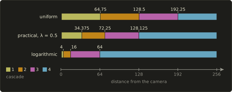
Now the ratios and the texel-to-pixel estimate:
| Scheme | worst texel/pixel | ||||
|---|---|---|---|---|---|
| uniform | 64.75 | 1.985 | 1.496 | 1.332 | 34.1 (cascade 1) |
| logarithmic | 4 | 4 | 4 | 4 | 2.11 (all) |
| practical, | 34.375 | 2.102 | 1.773 | 1.998 | 18.1 (cascade 1) |
With uniform splits, one shadow texel near the camera covers about 34 pixels: blocky shadows right in front of the player, while the last cascade wastes resolution (ratio , texels smaller than pixels).
The logarithmic split is perfectly balanced, but its first cascade covers only 1 to 4 m, so most of what the player looks at falls into the later cascades, and the tiny first slice is hard to fit tightly in light space.
The practical scheme sits in between, with as a tuning knob.
Note that the product of the four ratios is always , whatever the scheme: you can only move the quality around, not create it.
That's also why the near plane matters so much: pushing from 0.1 m to 1 m divides by ten.
Stable cascades
The light's frustum is refitted around the camera's slice every frame, so when the camera moves or turns, the texel grid moves by fractions of a texel, the casters are sampled at slightly different places, and shadow edges crawl and flicker: shimmering (シマリング, ちらつき).
Stable cascades fix it with two rules:
- Fit each cascade with a bounding sphere of its slice instead of a tight box. A sphere's size doesn't change when the camera turns, so the texel size stays constant.
- Snap the frustum's position in light space to whole texels, so the texel grid only ever moves by whole texels and every caster is rasterized exactly the same way.
Worked example. A cascade's bounding sphere has radius 32 m, so the map covers 64 m with 2048 texels: one texel is m.
If the frustum center lands at m in light space, that's texels; snapping takes texels, or m.
The sphere wastes some resolution (it is bigger than the slice), which is the price of stability.
Other details
Casters outside the camera's slice (a tall building between the sun and the slice) must still reach the shadow map, so their depths are clamped to the light frustum's near plane ("pancaking"), and the depth bias of section 11.4 must be scaled per cascade, because the texel size differs (chapter 19 covers depth bias with depth precision).
Alternatives exist (warped shadow maps, or virtual shadow maps that page in only the visible texels of a huge map), but cascades are the common baseline at the time of writing.
You built a single shadow map in OpenGL chapter 23; cascades are the same pass repeated with light matrices.
24.3 Soft shadows with PCSS
In section 11.1 we computed the width of a penumbra by similar triangles: for a light of width at height and an occluder edge at height , .
PCF (section 11.4) blurs every shadow by the same amount, which looks wrong: real shadows are sharp at the point of contact and get softer with distance (contact hardening).
Percentage-closer soft shadows (PCSS, パーセンテージクローサーソフトシャドウ), presented by Randima Fernando (NVIDIA) in 2005, estimate the penumbra width from the shadow map itself and then run PCF with a kernel of that size.
Three steps
Measure distances from the light, along its axis: to the receiver point and to the blocker.
With the light, blocker and receiver treated as parallel planes, chapter 11's formula becomes (substitute and )
PCSS evaluates it per pixel:
- Blocker search (ブロッカー探索). Look at a region of the shadow map around the receiver's texel and average the depths that are closer to the light than the receiver. That average is . If no texel is closer, the point is fully lit and we stop.
- Penumbra estimate (半影の推定). Compute with the formula.
- Filtering. Run PCF with a kernel whose width is , converted to shadow-map texels.
How big must the search region be?
Only blockers inside the pyramid from the receiver point to the light can shadow it.
Seen from the light's center, that pyramid's cross-section is largest close to the light; at the light camera's near plane (distance ) it is wide, which in shadow-map units is the search width.
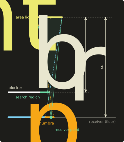
Worked example. We take chapter 11's numbers: a ceiling light 1 m wide at 4 m, the edge of a table at 1 m.
For a floor point near the table's shadow edge, .
The blocker search over, say, 16 texels finds 5 that are closer than 4, with depths 3.00, 3.00, 3.00, 2.90 and 3.10 (the table top, with a little noise), so
which is exactly the 0.33 m of section 11.1.
For the box lying on the floor (), m: a nearly hard shadow.
Now convert to texels.
If the spotlight's map has 1024 texels across the 8 m it covers on the floor, a texel is m there, and the table's penumbra needs a kernel texels wide.
A full 43 × 43 PCF would be 1849 lookups per pixel, so real implementations take 16 to 64 samples spread over the kernel (a Poisson disk or a rotated pattern) and denoise or blur the result.
For a directional light like the sun, the light width is replaced by its angular size: the sun's disc is about 0.53° across, so .
With the sun overhead, the shadow of the top of a 10 m lamp post has a penumbra of about 9 cm, while the base is sharp.
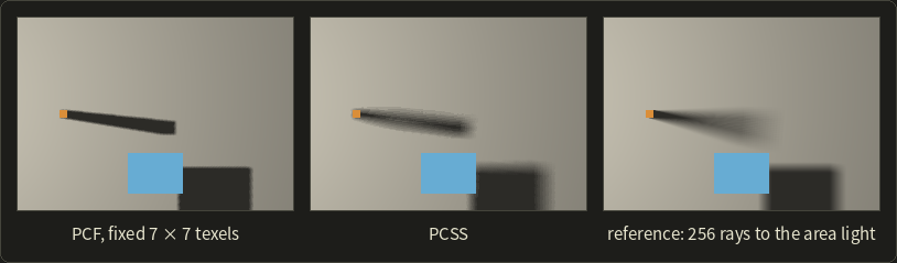
In the picture, the fixed PCF kernel gives the pole the same edge from its base to its tip, while PCSS and the reference both sharpen at the base and spread out at the tip.
PCSS is still an approximation: averaging the blocker depths treats all blockers as one plane, and a large search region on a tilted receiver can mistake the receiver itself for a blocker (the figure compares against the floor plane's own depth, a receiver-plane bias, to avoid that).
In a shader
Here is PCSS for a spotlight whose shadow map stores the linear depth along the light's axis (so the formula can use it directly).
lightSizeUv is the light's width divided by the width of the light frustum at its near plane, nearPlane that plane's distance; both searches use 7 × 7 samples.
// Percentage-closer soft shadows: 1 = fully lit, 0 = fully in shadow.
// The shadow map stores linear depth along the light's axis.
float pcss(Texture2D<float> shadowMap, SamplerState pointSampler, float2 uv, float zReceiver,
           float lightSizeUv, float nearPlane, float bias) {
  // 1. blocker search: the receiver-to-light pyramid, cut at the near plane
  float searchUv = lightSizeUv * (zReceiver - nearPlane) / zReceiver;
  float blockerSum = 0.0;
  int blockers = 0;
  for (int y = -3; y <= 3; ++y) {
    for (int x = -3; x <= 3; ++x) {
      float z = shadowMap.SampleLevel(pointSampler, uv + float2(x, y) * (searchUv / 6.0), 0);
      if (z < zReceiver - bias) {
        blockerSum += z;
        blockers += 1;
      }
    }
  }
  if (blockers == 0) return 1.0;
  // 2. penumbra width on the receiver, projected back to the near plane
  float zBlocker = blockerSum / float(blockers);
  float penumbraUv = lightSizeUv * (zReceiver - zBlocker) / zBlocker * nearPlane / zReceiver;
  // 3. PCF with that kernel
  float lit = 0.0;
  for (int y = -3; y <= 3; ++y) {
    for (int x = -3; x <= 3; ++x) {
      float z = shadowMap.SampleLevel(pointSampler, uv + float2(x, y) * (penumbraUv / 6.0), 0);
      lit += (zReceiver - bias > z) ? 0.0 : 1.0;
    }
  }
  return lit / 49.0;
}
// Percentage-closer soft shadows: 1 = fully lit, 0 = fully in shadow.
// The shadow map stores linear depth along the light's axis.
float pcss(sampler2D shadowMap, vec2 uv, float zReceiver, float lightSizeUv, float nearPlane,
float bias) {
// 1. blocker search: the receiver-to-light pyramid, cut at the near plane
float searchUv = lightSizeUv * (zReceiver - nearPlane) / zReceiver;
float blockerSum = 0.0;
int blockers = 0;
for (int y = -3; y <= 3; ++y) {
for (int x = -3; x <= 3; ++x) {
float z = textureLod(shadowMap, uv + vec2(x, y) * (searchUv / 6.0), 0.0).r;
if (z < zReceiver - bias) {
blockerSum += z;
blockers += 1;
}
}
}
if (blockers == 0) return 1.0;
// 2. penumbra width on the receiver, projected back to the near plane
float zBlocker = blockerSum / float(blockers);
float penumbraUv = lightSizeUv * (zReceiver - zBlocker) / zBlocker * nearPlane / zReceiver;
// 3. PCF with that kernel
float lit = 0.0;
for (int y = -3; y <= 3; ++y) {
for (int x = -3; x <= 3; ++x) {
float z = textureLod(shadowMap, uv + vec2(x, y) * (penumbraUv / 6.0), 0.0).r;
lit += (zReceiver - bias > z) ? 0.0 : 1.0;
}
}
return lit / 49.0;
}// Percentage-closer soft shadows: 1 = fully lit, 0 = fully in shadow.
// The shadow map stores linear depth along the light's axis.
float pcss(Texture2D<float> shadowMap, SamplerState pointSampler, float2 uv, float zReceiver,
float lightSizeUv, float nearPlane, float bias) {
// 1. blocker search: the receiver-to-light pyramid, cut at the near plane
float searchUv = lightSizeUv * (zReceiver - nearPlane) / zReceiver;
float blockerSum = 0.0;
int blockers = 0;
for (int y = -3; y <= 3; ++y) {
for (int x = -3; x <= 3; ++x) {
float z = shadowMap.SampleLevel(pointSampler, uv + float2(x, y) * (searchUv / 6.0), 0);
if (z < zReceiver - bias) {
blockerSum += z;
blockers += 1;
}
}
}
if (blockers == 0) return 1.0;
// 2. penumbra width on the receiver, projected back to the near plane
float zBlocker = blockerSum / float(blockers);
float penumbraUv = lightSizeUv * (zReceiver - zBlocker) / zBlocker * nearPlane / zReceiver;
// 3. PCF with that kernel
float lit = 0.0;
for (int y = -3; y <= 3; ++y) {
for (int x = -3; x <= 3; ++x) {
float z = shadowMap.SampleLevel(pointSampler, uv + float2(x, y) * (penumbraUv / 6.0), 0);
lit += (zReceiver - bias > z) ? 0.0 : 1.0;
}
}
return lit / 49.0;
}
The offsets run from to times a sixth of the width, so the 7 × 7 grid spans exactly one kernel width.
The cost is the problem: 98 lookups per pixel, many more for large lights.
That's why the next idea, shadow maps that can be pre-filtered like a texture, became popular.
24.4 Filterable shadow maps, contact shadows and ray-traced shadows
Chapter 11 showed (with the nine depths 0.35 and 0.62) that averaging depths before the comparison doesn't give soft shadows: the comparison is a step function, and filtering must happen after it.
So PCF can't use mipmaps, bilinear filtering of the stored values, or a cheap separable blur.
Filterable shadow maps store something else, something whose average still says how much of the texel area is lit.
Variance shadow maps
Variance shadow maps (VSM, 分散シャドウマップ; William Donnelly and Andrew Lauritzen, 2006) store two values per texel: the depth and its square .
After any linear filtering (blur, mipmap, bilinear), a texel holds the averages over its footprint, the first two moments of the depth distribution:
The lit fraction for a receiver at depth is the probability that a depth in the footprint is not in front of it.
We don't know the distribution, only its mean and variance, but the one-sided Chebyshev inequality (チェビシェフの不等式) gives an upper bound:
and for .
For a single flat occluder over a flat receiver the bound is exact, which is the common case at a shadow edge.
Worked example. Take chapter 11's nine stored depths (five of 0.35, four of 0.62) and a receiver at :
The true fraction (what PCF gives) is , and the bound is a little above it, as it must be.
The gain is that the VSM gets its two moments from one filtered lookup, whatever the filter size: a 43-texel blur costs the same as a 3-texel one when it is done once per frame on the map (separable Gaussian) or by mipmapping.
Light bleeding
The weak spot shows with two occluders.
Say half of a footprint holds depth 0.2 (a high blocker) and the other half 0.5 (a lower blocker), and the receiver at lies behind both: it should be fully dark.
A receiver just behind the lower blocker gets 36% of the light: a visible halo of light inside the shadow called light bleeding (光漏れ, ライトブリーディング).
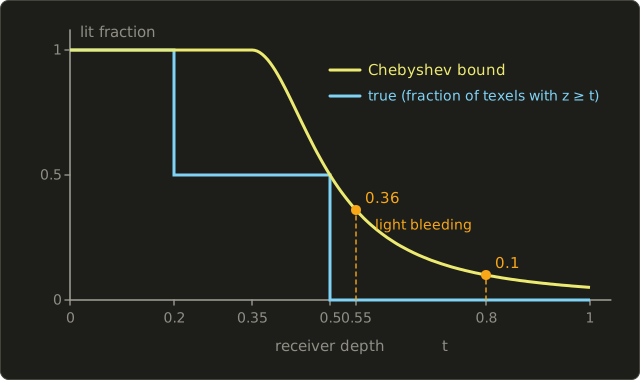
The usual cure is a light-bleeding reduction: remap from to and clamp, with around 0.2 to 0.4.
With , both 0.36 and 0.10 become 0, but every real penumbra also gets darker and narrower, so is again a tuning knob.
VSMs also need high precision (32-bit floats, because subtracts two nearly equal numbers) and twice the memory of a depth map.
Exponential and moment shadow maps
Exponential shadow maps (ESM, 指数シャドウマップ; Annen and colleagues, 2008) replace the step with an exponential.
For a receiver behind the occluder, is close to 0, and can be filtered linearly, so the map stores .
With depths in 0 to 1, the constant is limited by the float range: means , and around 80 is common.
With , a receiver 0.25 behind its occluder gets , dark, but one only 0.01 behind gets : ESM leaks light right at contact points.
Moment shadow maps (Christoph Peters and Reinhard Klein, 2015) store four moments, to , and reconstruct a tighter bound from them, with much less light bleeding at four values per texel.
Contact shadows
Shadow-map texels are centimeters wide, and the bias pushes shadows away from contact points (peter panning, section 11.4).
Contact shadows (コンタクトシャドウ) add a short screen-space ray march: from each pixel, take 8 to 16 small steps towards the light and compare each step's depth with the depth buffer; a step behind a visible surface means a close occluder.
It's cheap and fills in creases and the gap under a cup, but it only sees what is on screen, and it must assume a thickness for the depth buffer.
Ray-traced shadows and denoising
With hardware ray tracing (DXR, Vulkan ray tracing, at the time of writing on most desktop GPUs and current consoles), shadows can be computed exactly as in section 11.5: a shadow ray towards a random point on the area light.
One ray per pixel gives a correct but noisy penumbra (the Monte Carlo noise of chapter 23), so it's followed by a denoiser (デノイザー): a filter that averages each pixel with its neighbors in space (guided by depth and normals so that edges survive) and with its own history in time (reprojected with motion vectors, like the TAA of chapter 20).
Worked example. Temporal accumulation with an exponential moving average, with .
For independent samples of variance , the steady-state variance of is
so the history acts like 19 samples per pixel, at the cost of a lag (ghosting) when things move.
Ray-traced shadows have no acne from texel size, no cascades and no bias tuning, and their cost scales with the number of lights rather than with their size; their price is the rays and the denoiser.
24.5 Ambient occlusion in depth
Section 11.5 introduced ambient occlusion with rays: shoot rays into the hemisphere and count how many escape.
Now let's define it properly and see how games compute it from the depth buffer.
The definition
Ambient occlusion (AO, アンビエントオクルージョン, 環境遮蔽) at a point with normal is the cosine-weighted fraction of the hemisphere that is visible:
is 1 if a ray from in direction escapes (up to a maximum distance) and 0 if it hits something.
The normalizes, because (chapter 12).
Why the cosine?
Under a uniform sky of radiance , the irradiance is , so a Lambertian surface's radiance is exactly times its unoccluded value: AO is the exact answer for a uniform sky with no bounced light.
For anything else it's an approximation, which is why it's applied to the indirect (ambient) light only, never to the direct light, whose visibility the shadows already handle.
A variant, ambient obscurance (Zhukov and colleagues, 1998), replaces the binary by a function that grows with the hit distance, so faraway geometry darkens less; most game AO is really obscurance.
Worked example: why the cosine matters. Suppose the hemisphere is blocked all around below an elevation angle (a point at the bottom of a round pit), so the visible directions are those with angle from the normal.
With the cosine weighting,
For , : only a quarter of the ambient light is lost, because the blocked directions are the grazing ones, which contribute little.
Counting directions uniformly instead (the plain solid-angle fraction) gives : half.
When you sample AO with rays, cosine-weighted directions (chapter 23's importance sampling) make the estimator simply the fraction of rays that escape; with uniform directions, each ray must be weighted by its cosine.
Screen-space ambient occlusion
Screen-space ambient occlusion (SSAO, スクリーンスペースアンビエントオクルージョン), presented by Martin Mittring of Crytek in 2007 for Crysis, uses only the depth buffer:
- Reconstruct the view-space position of the pixel from its depth (chapter 19 derives the inverse projection).
- Take sample points in a small sphere of radius around it.
- Project each sample to the screen and read the depth buffer there. If the stored surface is in front of the sample (closer to the camera), the sample lies inside geometry: count it as occluded.
- , then blur the result to remove the noise.
Mittring's version sampled a full sphere and varied the sample pattern per pixel by reflecting it on a random plane read from a small texture.
A sphere has a known side effect: on a flat surface the lower half of the sphere is inside the floor, so a flat wall comes out about 50% occluded, which gives the gray, outline-heavy look of early SSAO.
Later versions sample a hemisphere oriented along the normal, which needs a normal buffer (as in deferred shading).
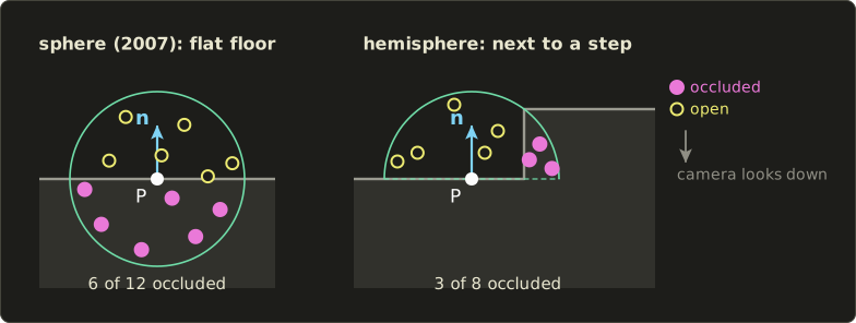
Worked example. In the left picture, 6 of 12 sphere samples lie under the flat floor: for an unoccluded floor.
In the right picture, the hemisphere next to a step 0.8 high has 3 of 8 samples inside the step: , a darkening that really is caused by the step.
A range check stops a foreground object from darkening the background far behind it (a halo), and the noise of the per-pixel rotations is removed by a small blur.
// Hemisphere SSAO for one pixel, in view space (the camera looks down -z, so larger z is closer).
// viewZ stores the view-space z of the visible surface; t, b, n form the pixel's tangent frame;
// kernel holds 16 offsets in the unit hemisphere around +z.
float ssao(Texture2D<float> viewZ, SamplerState pointSampler, float4x4 proj, float3 p,
           float3 t, float3 b, float3 n, float3 kernel[16], float radius) {
  float occluded = 0.0;
  for (int i = 0; i < 16; ++i) {
    float3 s = p + (t * kernel[i].x + b * kernel[i].y + n * kernel[i].z) * radius;
    float4 clip = mul(proj, float4(s, 1.0));
    float2 uv = clip.xy / clip.w * 0.5 + 0.5; // flip v here if the API's texture origin needs it
    float surfaceZ = viewZ.SampleLevel(pointSampler, uv, 0);
    float inRange = (abs(p.z - surfaceZ) < radius) ? 1.0 : 0.0;
    occluded += (surfaceZ > s.z + 0.02) ? inRange : 0.0;
  }
  return 1.0 - occluded / 16.0;
}
// Hemisphere SSAO for one pixel, in view space (the camera looks down -z, so larger z is closer).
// viewZ stores the view-space z of the visible surface; t, b, n form the pixel's tangent frame;
// kernel holds 16 offsets in the unit hemisphere around +z.
float ssao(sampler2D viewZ, mat4 proj, vec3 p, vec3 t, vec3 b, vec3 n, vec3 kernel[16],
float radius) {
float occluded = 0.0;
for (int i = 0; i < 16; ++i) {
vec3 s = p + (t * kernel[i].x + b * kernel[i].y + n * kernel[i].z) * radius;
vec4 clip = proj * vec4(s, 1.0);
vec2 uv = clip.xy / clip.w * 0.5 + 0.5; // flip v here if the API's texture origin needs it
float surfaceZ = textureLod(viewZ, uv, 0.0).r;
float inRange = (abs(p.z - surfaceZ) < radius) ? 1.0 : 0.0;
occluded += (surfaceZ > s.z + 0.02) ? inRange : 0.0;
}
return 1.0 - occluded / 16.0;
}// Hemisphere SSAO for one pixel, in view space (the camera looks down -z, so larger z is closer).
// viewZ stores the view-space z of the visible surface; t, b, n form the pixel's tangent frame;
// kernel holds 16 offsets in the unit hemisphere around +z.
float ssao(Texture2D<float> viewZ, SamplerState pointSampler, float4x4 proj, float3 p,
float3 t, float3 b, float3 n, float3 kernel[16], float radius) {
float occluded = 0.0;
for (int i = 0; i < 16; ++i) {
float3 s = p + (t * kernel[i].x + b * kernel[i].y + n * kernel[i].z) * radius;
float4 clip = mul(proj, float4(s, 1.0));
float2 uv = clip.xy / clip.w * 0.5 + 0.5; // flip v here if the API's texture origin needs it
float surfaceZ = viewZ.SampleLevel(pointSampler, uv, 0);
float inRange = (abs(p.z - surfaceZ) < radius) ? 1.0 : 0.0;
occluded += (surfaceZ > s.z + 0.02) ? inRange : 0.0;
}
return 1.0 - occluded / 16.0;
}Horizon-based AO and GTAO
Point samples waste information: a single depth buffer row already tells us the whole profile of the surface around the pixel.
Horizon-based ambient occlusion (HBAO; Louis Bavoil, Miguel Sainz and Rouslan Dimitrov, NVIDIA, 2008) marches along a few directions in screen space and finds, in each direction, the horizon angle: the highest elevation at which the depth buffer still blocks the view.
Everything below the horizon is occluded, everything above is open, so one march gives the visibility of a whole slice of the hemisphere.
HBAO integrates the visible part with uniform weighting; ground-truth ambient occlusion (GTAO; Jorge Jimenez, Xian-Chun Wu, Angelo Pesce and Adrian Jarabo, Activision, 2016) showed that the cosine-weighted integral within a slice has a closed form.
In a slice through the view direction, measure the two horizon angles from the normal (when the normal lies in the slice; GTAO also handles the general case with the angle between the normal's projection and the view vector).
With , the slice's visibility is
and the AO is the average of over the slice directions (2 to 4 per pixel, rotated every pixel and frame, then denoised).
Check it: an open hemisphere has , , and .
Horizons at 30° elevation on both sides mean , , and , the same as the pit above.
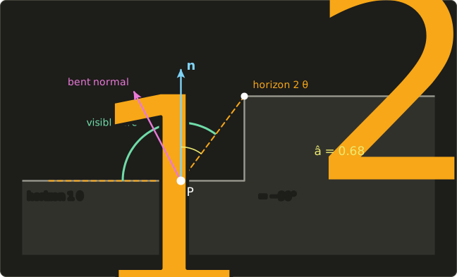
Worked example. In the figure, the left side is open () and the step's corner at sets the right horizon: , , and :
GTAO adds a multi-bounce fit (in bright corners light bounces between the walls, so plain AO darkens too much; a small cubic in and the albedo, fitted to ray-traced references, corrects it) and the bent normal (ベントノーマル): the average direction of the unoccluded part of the hemisphere, which in the figure leans about 28° away from the step.
Looking up irradiance with the bent normal makes the light come from where it actually can, and the cone of open directions gives a cheap specular occlusion for reflections.
Baked AO and ray-traced AO
For static objects, AO can be baked offline into an AO map (glTF 2.0's occlusion texture uses its red channel), which knows nothing about nearby objects.
Ray-traced AO (RTAO) shoots one or two short rays per pixel (AO is a near-field effect, so 0.5 to 2 m is typical) against the real scene and denoises: no screen-space limits, at the price of rays.
24.6 Baked global illumination and light probes
Now the bounced light itself.
The oldest real-time answer is to compute it offline: the radiosity or path tracing of chapter 12 runs once, and the result is stored.
Light maps
Light maps (section 11.10) store the precomputed irradiance of static surfaces in a texture with its own non-overlapping UVs.
Modern bakers compute them with GPU path tracers (chapter 23) and store more than one value per texel: a directional light map adds the dominant direction of the incoming light, or a few spherical-harmonics coefficients, so that normal maps still react to the baked light.
Light maps are perfect for walls and floors, but they can't light anything that moves, and they cost memory proportional to surface area.
Light probes
Moving objects (characters, vehicles, doors) are lit by light probes (ライトプローブ, chapter 12): sample points in space that store the light arriving there from all directions.
A probe stores a function on the sphere, and for diffuse lighting we only need its irradiance for every possible normal.
The standard compact representation is spherical harmonics.
Spherical harmonics
Spherical harmonics (SH, 球面調和関数) are to the sphere what sines and cosines are to a periodic signal: a basis of functions ordered by frequency.
They come in bands , with functions in band ; using bands 0 to gives functions, so "L1" means 4 and "L2" means 9.
Here are the real SH up to L2, as polynomials in the components of a unit direction.
We take as the polar ("up") axis to match our y-up convention; many references use , and the functions are the same with the letters swapped.
| Band | Functions | Constant |
|---|---|---|
| , , | ||
| , , | ||
They are orthonormal: is 1 for and 0 otherwise.
That makes projection easy, exactly like computing the coordinates of a vector with dot products in an orthonormal basis (Linear Algebra chapter 4):
In practice the integral is a sum over the texels of a cube map, each weighted by its solid angle, or a Monte Carlo estimate.
Why are 9 numbers enough for irradiance?
Irradiance is the radiance convolved with the clamped cosine , and convolving with a function that is symmetric around an axis just scales each band (the Funk–Hecke theorem).
Ravi Ramamoorthi and Pat Hanrahan (2001) computed the scale factors:
The factors drop fast (odd bands above 1 vanish entirely), so the cosine is a strong low-pass filter, and their paper showed that 9 coefficients give irradiance with an average error of about 1%.
Per color channel, that's 27 numbers per probe.
Worked example. A sky that is brightest at the zenith and black below the horizon: .
It is symmetric around , so only the "zonal" functions get nonzero coefficients.
Using over the upper hemisphere:
Reconstructing the radiance: L1 gives .
At the zenith that's 0.75 (true 1), at the horizon 0.25 (true 0) and at the nadir : a negative radiance, the SH version of the ringing of a truncated Fourier series.
L2 adds , giving 1.0625, 0.094 and 0.0625: better, but still visibly wrong.
Now the irradiance for a normal pointing up (), where the exact value is :
L2 is 0.8% low; L1 alone gives 1.8326, 12.5% low.
For a horizontal normal the exact irradiance is and L2 gives .
So 9 coefficients reproduce irradiance well even though they reproduce the radiance poorly.
That's the key point: SH probes are for diffuse light; sharp reflections need the reflection probes of section 24.7.
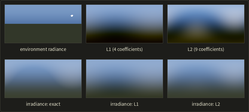
For the environment in the picture (a sky, a small bright sun and a dark ground), the L2 irradiance differs from the exact one by 1.5% on average and 6.1% at most, L1 by 7.0% on average and 23.7% at most.
The same projection and evaluation in C++:
#include <cmath>
#include <cstdio>
#include "linalg.hh"

// Real spherical harmonics up to L2, with y as the polar ("up") axis.
void shBasis(Vec3 d, float y[9]) {
  y[0] = 0.282095f;
  y[1] = 0.488603f * d.x;
  y[2] = 0.488603f * d.y;
  y[3] = 0.488603f * d.z;
  y[4] = 1.092548f * d.x * d.y;
  y[5] = 1.092548f * d.y * d.z;
  y[6] = 0.315392f * (3.0f * d.y * d.y - 1.0f);
  y[7] = 1.092548f * d.x * d.z;
  y[8] = 0.546274f * (d.x * d.x - d.z * d.z);
}

// Irradiance from 9 coefficients: E(n) = sum_l A_l c_lm Y_lm(n).
float shIrradiance(const float c[9], Vec3 n) {
  const float pi = 3.14159265f;
  const float a1 = 2 * pi / 3, a2 = pi / 4;
  const float a[9] = {pi, a1, a1, a1, a2, a2, a2, a2, a2};
  float y[9];
  shBasis(n, y);
  float e = 0;
  for (int k = 0; k < 9; ++k) e += a[k] * c[k] * y[k];
  return e;
}

int main() {
  // Project the sky L = max(y, 0) with a midpoint rule over theta (from +y) and phi.
  const float pi = 3.14159265f;
  const int nt = 256, np = 512;
  float c[9] = {};
  for (int i = 0; i < nt; ++i) {
    float th = (i + 0.5f) * pi / nt;
    for (int j = 0; j < np; ++j) {
      float ph = (j + 0.5f) * 2 * pi / np;
      Vec3 d{std::sin(th) * std::cos(ph), std::cos(th), std::sin(th) * std::sin(ph)};
      float dw = std::sin(th) * (pi / nt) * (2 * pi / np);
      float radiance = std::fmax(d.y, 0.0f);
      float y[9];
      shBasis(d, y);
      for (int k = 0; k < 9; ++k) c[k] += radiance * y[k] * dw;
    }
  }
  printf("c00 %.4f  c10 %.4f  c20 %.4f\n", c[0], c[2], c[6]);
  printf("E(up) %.4f  E(side) %.4f  E(down) %.4f\n", shIrradiance(c, {0, 1, 0}),
         shIrradiance(c, {1, 0, 0}), shIrradiance(c, {0, -1, 0}));
  return 0;
}
c00 0.8862  c10 1.0234  c20 0.4954
E(up) 2.0781  E(side) 0.6627  E(down) -0.0164
The small negative irradiance facing down is SH ringing again; engines clamp it or damp the higher bands slightly ("windowing").
PBR materials use this irradiance for their diffuse part; the specular part needs prefiltered environment maps (chapter 22).
Irradiance volumes and probe grids
Where should the probes be?
The irradiance volume (Greger, Shirley, Hubbard and Greenberg, 1998) puts them on a regular 3D grid; artists or tools may also place them by hand, densely where the light changes and sparsely in open space.
A point between probes interpolates the eight probes of its grid cell trilinearly: with fractional position inside the cell, the probe at corner gets the weight
Worked example. : corner gets , corner gets , corner gets , and the eight weights sum to 1.
The interpolated SH coefficients (a linear combination of the probes' coefficients) are then evaluated with the normal as above.
The classic artifact is light leaking (光漏れ).
A wall between two probes doesn't stop the interpolation, so a point in a dark room next to a sunlit room picks up the bright probe behind the wall, and the dark room glows along the wall.
In the left picture the bright probes leak through the wall into the dark room (and the dark ones darken the bright side); on the right each probe's weight is multiplied by a visibility test (Chebyshev on stored distances, see DDGI in section 24.8), and the wall separates the rooms again.
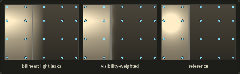
Simpler fixes: place probes so that no cell straddles a wall, down-weight probes behind the surface, or offset the lookup along the normal.
24.7 Reflections: probes and screen space
Glossy and mirror reflections need much more angular detail than irradiance, so SH is not enough.
Reflection probes with parallax correction
A reflection probe (リフレクションプローブ) is a cube map captured at one point of the scene and prefiltered for several roughness levels (chapter 22; you build them in OpenGL chapter 24).
Section 11.9 warned that environment maps assume the surroundings are infinitely far away.
Inside a room that's badly wrong: a point near the right wall looks up the probe with its reflection direction as if it stood at the probe's position, and sees the wrong part of the room.
Parallax correction (視差補正) fixes it with a simple proxy of the room, usually a box: intersect the reflection ray from the shading point with the box, and look up the cube map in the direction from the probe to that hit point.
The idea appeared in GPU Gems (Kevin Bjorke, 2004) and was popularized for games by Sébastien Lagarde and Antoine Zanuttini (SIGGRAPH 2012).
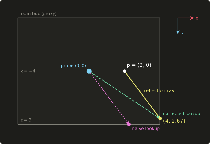
Worked example (seen from above, so only and ).
The room box spans , ; the probe is at the origin; the point is with reflection direction .
The ray leaves the box through the nearest exit plane, so take the smaller of the two exit distances:
The corrected lookup direction is , normalized , which differs from by 19.4°.
The naive lookup with from the probe would show the wall point , almost 2 m away from the right one.
The box is only a proxy, so furniture still reflects in the wrong place, and points near the probe's position get the best results; engines blend several overlapping probes.
Screen-space reflections
Screen-space reflections (SSR, スクリーンスペースリフレクション) trace the reflection ray through the depth buffer instead: march along the ray's projection on the screen (often accelerated with a min-depth pyramid, "Hi-Z"), and where the ray passes behind the depth buffer, reuse that pixel's lit color.
It's accurate for things on screen (wet streets reflecting neon signs), but it can't reflect what isn't on screen (the sky behind the camera, hidden surfaces), so it fades out near the screen edges and falls back to reflection probes.
Screen-space GI (SSGI) uses the same marching for diffuse bounces with many short rays per pixel, with the same blind spots.
24.8 Dynamic global illumination
Baked light can't follow a door that opens or a sun that sets.
Dynamic GI recomputes (some of) the bounced light every frame.
Reflective shadow maps
The first bounce of a light starts at the surfaces that the light directly illuminates, and those are exactly what the shadow map sees.
Reflective shadow maps (RSM, 反射シャドウマップ; Carsten Dachsbacher and Marc Stamminger, 2005) store, besides depth, the world position, the normal and the reflected flux of every texel; each texel then acts as a small light, a virtual point light (VPL, 仮想点光源), for the rest of the scene.
A texel of a Lambertian surface with reflected flux , position and normal emits like a tiny radiosity patch (chapter 12): its intensity in a direction at angle from its normal is , so the irradiance it adds at a point with normal is
Worked example. A 10 cm × 10 cm floor texel with albedo 0.8 in sunlight of irradiance 1 W/m² reflects W.
At with , it lights a wall point with .
The distance is , both cosines are , and
Summing a few hundred such texels per pixel (sampled with importance around the pixel's projection into the map) gives the first bounce, with the color of the reflecting surfaces: real-time color bleeding.
RSMs ignore visibility between the VPL and the receiver, so light passes through walls; light propagation volumes (LPV; Anton Kaplanyan, Crytek, 2009) inject the VPLs into a coarse 3D grid of SH coefficients and propagate the light from cell to cell, which can respect a coarse occlusion grid.
Voxel cone tracing
Voxel cone tracing (VCT, ボクセルコーントレーシング; Cyril Crassin, Fabrice Neyret, Miguel Sainz, Simon Green and Elmar Eisemann, 2011; later shipped by NVIDIA as VXGI) voxelizes the scene each frame (or updates it incrementally) into a 3D texture of the light leaving each voxel, with a full mipmap pyramid.
Instead of many rays, it traces a few cones: for diffuse light, a handful of wide cones covering the hemisphere; for glossy reflections, one narrow cone.
Along a cone, the footprint grows with distance, so the shader samples coarser and coarser mip levels and composites them front to back like the volume rendering of chapter 28.
Worked example. Voxels of 0.25 m and a cone with a 60° aperture: at distance the cone is wide, and the mip level whose voxels match it is .
At m that's ; at m, 4.21; each doubling of the distance adds exactly one level.
So a cone reaches far with a few samples, which is the method's strength; its weaknesses are the cost of keeping the voxels up to date and the leaking that coarse voxels cause through thin walls.
DDGI: probes updated by ray tracing
Dynamic diffuse global illumination (DDGI; Zander Majercik, Jean-Philippe Guertin, Derek Nowrouzezahrai and Morgan McGuire, 2019) keeps the probe grid of section 24.6 but updates every probe every frame with ray tracing:
- Each probe shoots a few dozen to a few hundred rays (the paper tested 32 to 256) in a randomly rotated spiral pattern, shading the hit points with direct light plus the previous frame's probes, so light keeps bouncing from frame to frame.
- It stores irradiance in a small octahedral map (8 × 8 texels) and, in a second map (16 × 16), the mean distance and mean squared distance to the hits in each direction.
- New results are blended in with a hysteresis (the paper uses 0.85 to 0.98): .
The distance moments are a variance shadow map seen from the probe.
When shading a point, each of the eight surrounding probes checks with Chebyshev's inequality whether the point could be visible from the probe, and its weight is reduced if not: that is what stops the leaking in the probe-grid picture.
Worked example. A probe's mean distance towards a point is m with mean squared distance 4.1, so .
The point is 3.0 m away, so a wall probably lies between them: , and the probe's weight drops to 9%.
For the hysteresis, take and a light that suddenly switches on: after frames the probes reach of the new value, 51% after 14 frames and 90% after 45 frames (0.75 s at 60 fps).
At the time of writing, NVIDIA distributes DDGI in its RTXGI SDK.
24.9 Ray-traced GI, ReSTIR and hybrid pipelines
With hardware ray tracing, the honest approach of chapter 12 becomes possible: trace a few rays per pixel, bounce once or twice, denoise.
The challenge is the sample budget, often one or two rays per pixel, so which sample each ray takes becomes everything.
The most influential idea of recent years is to let pixels share their good samples.
Resampled importance sampling
Take direct lighting from many lights first.
For a pixel, the ideal light sample would be drawn with probability proportional to the light's actual contribution (chapter 23's importance sampling), but includes visibility, which costs a ray per light.
Resampled importance sampling (RIS) works in two stages:
- Draw cheap candidates from a simple source distribution (for example, a uniformly chosen light).
- Give each a weight , where is a target function that is cheap but close to (the light's contribution without the shadow ray), and pick one candidate with probability .
Then trace one shadow ray to only, and use the estimator
where plays the role of for the chosen sample.
The candidates can be picked one by one without storing them, with weighted reservoir sampling (リザーバサンプリング): keep the current choice, the running sum and the count ; for each new candidate with weight , add it to and replace the choice with probability .
In the end every candidate has been kept with probability exactly .
Worked example. The scene has 100 lights, so .
Four candidates have target values , so weights , and the random numbers are :
| Candidate | Kept? | ||||
|---|---|---|---|---|---|
| 1 | 2 | 2 | 1 | 0.7 | yes |
| 2 | 30 | 32 | 0.9375 | 0.4 | yes, replaces 1 |
| 3 | 5 | 37 | 0.1351 | 0.6 | no |
| 4 | 13 | 50 | 0.26 | 0.9 | no |
The reservoir holds candidate 2, with .
If the shadow ray finds the light visible, and the estimate is : exactly , the average of the candidates' , which is an estimate of the total unshadowed light .
The probabilities of ending with candidates 1 to 4 were = 0.04, 0.6, 0.1, 0.26: the strong light wins most of the time, and only one shadow ray was traced.
ReSTIR: reuse in space and time
ReSTIR (Spatiotemporal Reservoir Resampling; Benedikt Bitterli, Chris Wyman, Matt Pharr, Peter Shirley, Aaron Lefohn and Wojciech Jarosz, SIGGRAPH 2020) observes that a reservoir is itself a summary of candidates, and reservoirs can be merged: treat another reservoir's chosen sample as one candidate whose weight is , and add its count .
Each frame, every pixel:
- builds a fresh reservoir from a few candidates;
- merges the reservoir of the same surface point in the previous frame (temporal reuse, found with motion vectors);
- merges the reservoirs of a few random neighboring pixels (spatial reuse), re-evaluating at its own position, because a light that's strong for the neighbor may be weak here.
After a few frames, each pixel effectively chooses among thousands of candidates while tracing one or two shadow rays.
The paper rendered scenes with up to 3.4 million emissive triangles in real time and reported equal error 6 to 60 times faster than the previous state of the art.
Two cautions: the temporal count must be capped (often at about 20 times the per-frame count), or the history dominates and the image reacts sluggishly; and naive merging is biased when neighbors see different geometry, so the paper gives a cheaper biased and a careful unbiased version.
The same idea applied to bounce paths, ReSTIR GI (Ouyang and colleagues, 2021), resamples the hit points of indirect rays, which makes path-traced GI with one path per pixel usable after denoising.
Hybrid pipelines at the time of writing
Real engines combine several of these methods; a few examples (products change quickly; the ideas are what matter):
- Unreal Engine 5's Lumen keeps a surface cache (サーフェスキャッシュ): mesh surfaces captured from several directions ("cards") whose lighting is updated over several frames, so a ray hit looks up lighting instead of shading from scratch. Rays first try the screen, then software ray tracing against signed distance fields (chapter 21), or hardware ray tracing where supported.
- Probe-based GI with DDGI-style ray-traced probes (for example NVIDIA's RTXGI) for diffuse light, with reflection probes or ray-traced reflections for the specular part.
- Path-traced modes in some games, such as the "RT: Overdrive" mode of Cyberpunk 2077 (2023), which uses NVIDIA's RTXDI, an implementation of ReSTIR, for its many lights, together with denoising and upscaling (chapter 29).
A typical frame may still combine cascaded shadow maps with contact shadows, GTAO, baked light maps, probes for characters, and SSR with probe fallback.
24.10 Comparing the techniques
| Technique | Computes | Dynamic? | Cost | Typical artifacts |
|---|---|---|---|---|
| Cascaded shadow maps | sun visibility | fully | N depth passes | shimmering, seams, bias tuning |
| PCSS | soft shadow visibility | fully | blocker search + large PCF | wrong with layered blockers, cost |
| VSM / ESM / MSM | filterable visibility | fully | 2–4 values per texel | light bleeding / contact leaks |
| Ray-traced shadows | exact visibility | fully | rays per light + denoiser | noise, ghosting |
| SSAO / HBAO / GTAO | near-field sky visibility | fully | a few ms or less, screen space | halos, missing off-screen occluders |
| Light maps | diffuse GI on static surfaces | no (baked) | memory, bake time | can't light moving objects |
| SH probes / irradiance volumes | diffuse GI at points | baked or updated | 9 values × 3 per probe | leaking, low frequency only |
| Reflection probes (parallax-corrected) | glossy reflections | baked or re-captured | cube maps | wrong parallax away from proxy |
| SSR / SSGI | reflections / bounce from screen | fully | screen-space marching | missing off-screen content |
| RSM / LPV | first diffuse bounce | fully | VPL sums / grid propagation | no or coarse visibility, leaks |
| Voxel cone tracing | diffuse and glossy GI | fully | voxelization + cones | leaking, voxel cost |
| DDGI | diffuse GI, multi-bounce | fully | rays per probe | lag (hysteresis), probe placement |
| Ray-traced GI + ReSTIR | direct and indirect light | fully | 1–2 rays per pixel + denoiser | noise, temporal artifacts |
Exam points
These tie back to the syllabus items shadowing (chapter 11) and global illumination (chapter 12):
- The penumbra width grows with the distance between blocker and receiver, : soft shadows are sharp at contact points. PCF alone blurs by a fixed amount; PCSS estimates the width from the average blocker depth.
- Shadow-map filtering must happen after the comparison (PCF), unless the map stores something filterable (VSM moments).
- Ambient occlusion is the visible fraction of the hemisphere, cosine-weighted; it darkens the ambient (indirect) light only.
- Light maps store precomputed lighting of static surfaces; light probes store the light at points in space for moving objects; environment (reflection) maps assume distant surroundings.
- Radiosity-style diffuse GI is view independent and can be baked; specular effects depend on the view and need per-frame methods (probes, SSR, ray tracing).
24.11 Summary
- Cascaded shadow maps split the view; logarithmic splits balance perspective aliasing, the practical scheme blends them with uniform splits by ; bounding spheres and texel snapping stop shimmering.
- PCSS finds the average blocker depth, estimates the penumbra and runs PCF of that width, giving contact-hardening soft shadows.
- VSMs store and , can be blurred, and use Chebyshev's bound ; layered occluders cause light bleeding. ESM, moment shadow maps, contact shadows and denoised ray-traced shadows complete the toolbox.
- AO is ; SSAO samples the depth buffer, HBAO finds horizons, GTAO integrates each slice analytically; AO can also be baked or ray traced.
- Light maps bake static GI; SH probes store irradiance in 9 coefficients per channel thanks to the cosine's low-pass factors ; probe grids interpolate trilinearly and leak without visibility weights.
- Reflection probes need parallax correction with a proxy box; SSR and SSGI reuse the screen but can't see off-screen content.
- RSMs turn shadow-map texels into virtual point lights, voxel cone tracing samples a voxel mip pyramid, DDGI updates probes by ray tracing with Chebyshev visibility.
- ReSTIR picks samples by resampled importance sampling with reservoirs and shares them across pixels and frames.
24.12 Key terms
| English | 日本語 |
|---|---|
| direct light, indirect light | 直接光、間接光 |
| baking, baked lighting | ベイク(事前計算した照明) |
| cascaded shadow maps (CSM) | カスケードシャドウマップ(CSM) |
| perspective aliasing | 透視エイリアシング |
| uniform, logarithmic, practical split scheme | 均等分割、対数分割、実用分割方式 |
| shimmering | ちらつき(シマリング) |
| stable cascades, texel snapping | 安定カスケード、テクセル単位のスナップ |
| percentage-closer soft shadows (PCSS) | PCSS(パーセンテージクローサーソフトシャドウ) |
| blocker search | ブロッカー探索 |
| penumbra estimation | 半影の推定 |
| contact hardening | コンタクトハードニング |
| variance shadow map (VSM) | 分散シャドウマップ(VSM) |
| moment | モーメント(積率) |
| Chebyshev's inequality | チェビシェフの不等式 |
| light bleeding | 光漏れ(ライトブリーディング) |
| exponential shadow map (ESM) | 指数シャドウマップ(ESM) |
| moment shadow map | モーメントシャドウマップ |
| contact shadow | コンタクトシャドウ |
| denoiser, temporal accumulation | デノイザー、時間方向の蓄積 |
| ambient occlusion (AO) | アンビエントオクルージョン(環境遮蔽) |
| ambient obscurance | アンビエントオブスキュランス |
| screen-space ambient occlusion (SSAO) | スクリーンスペースアンビエントオクルージョン(SSAO) |
| horizon-based ambient occlusion (HBAO) | 地平線ベースのアンビエントオクルージョン(HBAO) |
| ground-truth ambient occlusion (GTAO) | GTAO |
| horizon angle | 地平線角 |
| bent normal | ベントノーマル |
| specular occlusion | スペキュラーオクルージョン |
| light map, directional light map | ライトマップ、指向性ライトマップ |
| light probe | ライトプローブ |
| spherical harmonics (SH) | 球面調和関数(SH) |
| band | バンド(次数) |
| irradiance, radiance | 放射照度、放射輝度 |
| irradiance volume | イラディアンスボリューム |
| trilinear interpolation | 3線型補間 |
| light leaking | 光漏れ |
| reflection probe | リフレクションプローブ(反射プローブ) |
| parallax correction | 視差補正 |
| screen-space reflections (SSR) | スクリーンスペースリフレクション(SSR) |
| screen-space global illumination (SSGI) | スクリーンスペースGI(SSGI) |
| reflective shadow map (RSM) | 反射シャドウマップ(RSM) |
| virtual point light (VPL) | 仮想点光源(VPL) |
| light propagation volumes (LPV) | ライトプロパゲーションボリューム(LPV) |
| voxel cone tracing | ボクセルコーントレーシング |
| dynamic diffuse global illumination (DDGI) | DDGI |
| hysteresis | ヒステリシス |
| resampled importance sampling (RIS) | リサンプル重点的サンプリング(RIS) |
| weighted reservoir sampling | 重み付きリザーバサンプリング |
| ReSTIR | ReSTIR |
| surface cache | サーフェスキャッシュ |
24.13 Challenges
- ★ Compute the uniform, logarithmic and practical () split distances for , and , and the ratio of every cascade. Which cascade limits the quality in each scheme?
- ★ An area light 0.6 m wide shines on a floor 5 m from it. The blocker search under a chair finds an average blocker distance of 4 m; under a book lying on the floor, 4.9 m. Compute both penumbra widths, and their sizes in texels if a texel covers 1 cm at the floor.
- ★★ A 3 × 3 VSM footprint holds six texels of depth 0.4 and three of depth 0.7. Compute , and , then for receivers at and at . Compare with the true lit fraction in both cases and explain which result is light bleeding.
- ★★ A GTAO slice with has horizons and . Compute and the contribution of each side. Which side loses more of its half, and why does a high horizon cost more than its angle suggests?
- ★★★ Run a 4-candidate reservoir by hand: 50 lights picked uniformly, target values , random numbers . Which light is kept, what are and the estimate if the light is visible, and what is the probability of keeping each candidate? Then explain why a spatial neighbor's reservoir must be re-weighted with this pixel's before merging, and why the temporal is capped.
Multiple choice
Q1 ★ Which of the following statements about real-time shadow techniques is correct?
| A | With uniform cascade splits, every cascade has the same ratio of far to near distance, which is the ideal against perspective aliasing. |
| B | Variance shadow maps store only the mean depth, so they can't be blurred before the shadow test. |
| C | PCF with a fixed kernel widens the penumbra correctly with the distance between blocker and receiver. |
| D | PCSS averages the depths of the blockers found in a search region and estimates the penumbra width from the light size and the blocker and receiver distances, so shadows stay sharp near contact points. |
| E | Snapping the light's frustum to whole texels makes cascades shimmer more when the camera moves. |
Q2 ★★ Which of the following statements about ambient occlusion is correct?
| A | Ambient occlusion depends on the positions of the light sources, so it changes whenever a light moves. |
| B | The SSAO of Crysis (2007) traced rays against the scene's triangles with ray-tracing hardware. |
| C | GTAO finds two horizon angles in each screen-space slice and computes the cosine-weighted visibility within the slice analytically, so only the slice directions are sampled. |
| D | With cosine weighting, a horizon at 30° elevation all around blocks half of the ambient light. |
| E | Baked AO maps are normally multiplied with the direct sunlight to create cast shadows. |
Q3 ★★ Which of the following statements about real-time global illumination is correct?
| A | The irradiance from a distant environment is approximated well by spherical harmonics up to L2 (9 coefficients per color channel), because convolution with the clamped cosine strongly damps the higher bands. |
| B | Reflective shadow maps compute indirect light by tracing rays from the camera through a voxel grid. |
| C | DDGI probes store only irradiance and never test visibility, so light leaking through walls can't be reduced. |
| D | Screen-space reflections can reflect objects that are outside the screen or hidden behind other objects. |
| E | ReSTIR traces a shadow ray to every light in the scene every frame and then keeps the brightest one. |
24.14 Practical assignment
Light a small scene by hand: plan the cascades for its camera, measure the ambient occlusion of a point from a drawing, and build an L1 light probe from six numbers.
You need graph paper, a ruler, a protractor, a pencil, two colored pens and a calculator.
Part A: cascades.
The camera sees from m to m and uses cascades.
- Compute the uniform, logarithmic and practical () split distances.
- Draw three horizontal bars from 0 to 162 m (1 cm = 10 m) and mark the splits of each scheme, like the figure in section 24.2.
- Ratios. For every cascade compute and the rough texel-to-pixel factor of section 24.2. Circle the worst cascade of each scheme.
Part B: ambient occlusion from a drawing.
A side view (x to the right, y up, 1 unit = 2 cm): a floor , the point with normal , a low box on the left with its top corner nearest to at (the box covers , ), and a wall on the right that starts at and is 2 high. The AO radius is 3.
- Draw the scene, the half circle of radius 3 around , and the two horizon lines from to the corners and . Check that both corners lie inside the radius.
- Measure both horizon elevations with the protractor, then compute them with , and convert them to angles from the normal, .
- Compute the slice visibility with the GTAO formula (). Then shade the visible arc with the first pen and draw the bent normal by eye, leaning towards the more open side.
Part C: an L1 light probe from six directions.
A probe measured the radiance in the six axis directions: 3 from (sky), 1 from (ground) and 2 from each of and .
Treat the six values as samples of the sphere, each standing for a solid angle of .
- Project: , and (and the same for and ), where is the y component of direction .
- Reconstruct the radiance in the six directions from the four coefficients, and the irradiance for normals pointing up, down and sideways.
- Leak check. The probe lies at in a corridor; a second probe at , in a brightly lit room, has irradiance 30, and a wall stands at between them, with a point to shade at . Use your sideways irradiance as the value of the probe at , interpolate linearly between the two probes, and then repeat with the far probe's weight multiplied by a visibility factor 0.1 (renormalizing the weights).
How to check yourself:
- Part A: the product of the four ratios is in every scheme; the logarithmic splits are 2, 6, 18, 54, 162 with every ratio equal to 3.
- Part B: the left horizon is at elevation and the right one at 45°; because , exactly, and comes out as a round number between 0.6 and 0.7.
- Part C: the six values are exactly the linear function , so the L1 reconstruction must give back all six values, and the irradiance must equal .
- Part C: the visibility-weighted result must lie much closer to the near probe's value than the plain interpolation does.
コメント(0)
まだコメントはありません。
ログインするとコメント出来ます。