25. Advanced Character Animation
Chapter 13 built a character: a skeleton of joints, forward and inverse kinematics, a skin attached with linear blend skinning, blend shapes for the face, and motion capture to feed it.
Chapter 14 made it run in a game: clips blended and cross-faded, state machines, blend trees, ragdolls and crowds.
This chapter opens those boxes.
We'll start with the skin.
Chapter 13 showed that linear blend skinning makes elbows thin and twisted wrists collapse, and promised the fix: dual quaternion skinning, which we'll derive and compute here, together with the corrective shapes and smoothing deformers that clean up what is left.
Then we'll go deeper into blending: blend spaces with worked weights, additive and layered animation, root motion, and inertialization, a cheaper and better transition than the cross-fade.
Next comes motion matching, the technique that replaced hand-built state machines in many recent games, with a worked search.
Then full-body inverse kinematics: FABRIK, the Jacobian methods with a worked step, joint limits, feet on uneven ground, heads that look at things, and physically powered ragdolls.
We finish with faces solved from performance capture, crowds, and how animation data is compressed.
All of this is beyond the exam syllabus, but it grows directly out of two syllabus items of area 5, character animation (キャラクタのアニメーション) and real-time animation (リアルタイムアニメーション), and the exam points near the end of section 25.6 tie it back to them.
The math is the quaternion algebra of Linear Algebra chapter 13 and the transformation matrices of this series' chapters 4 and 5; I'll link back instead of re-teaching them.
25.1 Skinning matrices, worked in full
The chain of matrices
Recall the formula of linear blend skinning (LBS, リニアブレンドスキニング) from chapter 13, section 13.8:
Three matrices meet in it, and each comes from a different place:
- , the bone's world matrix in the bind pose (バインドポーズ), the pose the mesh was modeled in. It never changes, so the engine stores its inverse, the inverse bind matrix (逆バインド行列), in the model file (glTF calls the array
inverseBindMatrices). - , the bone's world matrix in the current pose, computed every frame by forward kinematics from the animated local transforms: .
- , the skinning matrix, the product of the two: "undo where the bone was when the mesh was modeled, then do where the bone is now".
Why the inverse bind matrix?
A vertex is stored in model space, not relative to any bone.
If we applied alone, a vertex near the elbow would be moved by the elbow's whole offset from the origin a second time.
first expresses the vertex in the bone's own frame, and carries that frame to its new place.
A useful check follows immediately: in the bind pose , so every and the mesh stays exactly where it was modeled, whatever the weights are.
Worked example
Take the two-bone arm of chapter 13 in 2D, with the homogeneous 3 × 3 matrices of chapter 4.
Bone 0 starts at the origin, bone 1 at , so and .
This time both joints move: the shoulder turns by 30° and the elbow by 90° relative to the upper arm:
The skinning matrices are and .
Read right to left: move the elbow to the origin, turn by 90°, move it back, then turn the whole arm by 30° about the shoulder.
Multiplied out,
Now skin the vertex on the outside of the elbow, , with the weights 0.5 and 0.5:
- ;
- ;
- blended: .
The elbow is now at , and the vertex is from it: the same thinning to 0.354 as in chapter 13, because turning the whole arm doesn't change the shape of the bend.
Why the skin shrinks: the blended matrix
Since the blend is linear, we can blend the matrices first and apply the result once:
Its upper-left 2 × 2 part has the determinant , and it is : a rotation by 75°, halfway between 30° and 120°, times a uniform scale of 0.707.
That's a general identity worth remembering:
The average of two rotations points the right way but shrinks by the cosine of half the angle between them: 0.707 at 90°, 0 at 180°.
It's the matrix lerp of chapter 13, section 13.4 again, now hidden inside every skinned vertex near a joint.
So LBS isn't wrong because of the weights; it's wrong because a weighted sum of rigid transforms is not a rigid transform.
In practice
The skinning matrices of a rigid skeleton have the bottom row , so the matrix palette is usually uploaded as 3 × 4 matrices: 12 floats per joint instead of 16.
Normals use the blended 3 × 3 parts, which is exact only without scaling; a scaled bone needs the inverse transpose of chapter 5, section 5.4.
25.2 Dual quaternion skinning
The fix for the shrinking is to blend something that stays rigid.
For rotations alone we already know the answer: blend unit quaternions and normalize (nlerp), and the result is always a rotation (Linear Algebra chapter 13, section 13.6).
But a bone turns about its own joint, not about the origin, so its rotation and translation belong together; blending them separately rotates about the wrong center.
Dual quaternions (デュアルクォータニオン, 双対四元数) put rotation and translation into one object that can be blended and normalized like a quaternion.
Kavan, Collins, Žára and O'Sullivan introduced dual quaternion skinning (DQS, デュアルクォータニオンスキニング) in "Skinning with Dual Quaternions" (I3D 2007) and analyzed it fully in "Geometric Skinning with Approximate Dual Quaternion Blending" (ACM Transactions on Graphics, 2008).
Dual numbers
A dual number (双対数) is , where is a new symbol with the single rule
That's all; compare complex numbers, where .
Multiplying two dual numbers, the term simply drops out:
For example .
Dual quaternions and rigid transforms
A dual quaternion is the same idea with quaternions as the parts:
is the real part and the dual part, each an ordinary quaternion ; that's 8 numbers.
Products follow the dual number rule with the Hamilton product of Linear Algebra chapter 13:
A rigid transform "rotate by the unit quaternion , then translate by " is the unit dual quaternion
and its product with another unit dual quaternion is the composition of the two transforms, exactly like multiplying matrices.
To apply it to a point , we rotate with the real part and read the translation back from the dual part:
(since for a unit ).
Blending: dual quaternion linear blending
DQS replaces the blended matrix of LBS by a blended dual quaternion, dual quaternion linear blending (DLB):
- The weights are the same skin weights as for LBS; nothing in the rig changes.
- picks the sign: and are the same rotation (the double cover, Linear Algebra section 13.5), and we take the sign for which , so that all bones of a vertex blend "the short way round", as slerp does.
- Both parts are divided by the length of the blended real part. Then is a unit quaternion, a pure rotation, and the vector part of is a translation: whatever the weights, the vertex is moved by a rigid transform. (A tiny leftover in the scalar part of is simply ignored.)
Worked example: the bent elbow
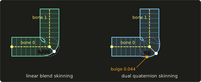
Same bend as in chapter 13: bone 1 turns by 90° about z around the elbow , bone 0 stays, and the vertex has the weights 0.5 and 0.5.
Bone 1 as a dual quaternion. The rotation is .
A rotation about the point is "rotate about the origin, then translate by ": , so .
The dual part is .
For two quaternions ; here and
so .
Bone 0 is the identity, and .
Blend. , so no sign flip.
The real part is a rotation by 45°, exactly half of the bend.
Translation. Write and . The vector part of works out to .
With , , and :
And that is : the blended transform is a rotation by 45° about the elbow.
The vertex. , plus , gives , at the distance from the elbow.
LBS put it at , 0.354 from the elbow; DQS keeps the full radius of the tube.
Worked example: twisting, and the flip
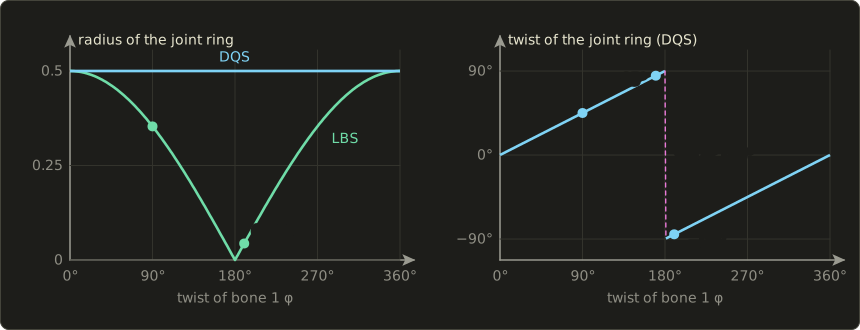
Now the candy wrapper of chapter 13: bone 1 twists by about the x axis (the bone's own axis), and we follow the vertex on the ring at the joint, weights 0.5 and 0.5.
The twist axis passes through the origin, so there is no translation, and .
- : , normalized , a twist of 45°. The vertex goes to , radius 0.5. LBS: radius .
- : , dot with positive; the blend is a twist of 85°, radius 0.5. LBS: , nearly collapsed.
- : , and now the dot product is negative, so is used: the same rotation, described as a twist of . The blend is a twist of .
The radius is always 0.5: no candy wrapper.
But between 170° and 190° the ring at the joint jumps from to , a sudden turn of 170° for a smooth 20° change of the bone.
That's the flipping artifact Kavan and colleagues describe: DQS always blends the short way round, and at 180° the short way switches sides (at exactly 180° the dot product is 0 and rounding decides).
LBS has its own version: its ring passes through radius 0 at 180°.
Real rigs avoid such large twists on one joint anyway, with twist bones that share the rotation.
Bulging
In the bent tube, vertices a little before the joint have a small weight on bone 1 and are turned by a small angle about the elbow, which swings them outward.
With the weights of chapter 13 (fading from 0 at to 1 at ), the outside sticks out to , 0.044 beyond the upper arm's surface at : a bulge (膨らみ) of about 9 % of the radius, where LBS collapses inward.
It is usually accepted or fixed with a corrective shape (section 25.3); some DCC tools also blend LBS and DQS per vertex (Maya's skin cluster, for example, offers "Classic Linear", "Dual Quaternion" and a weight-blended mix).
In code
Here are DLB and the two worked examples in C++, with Quat, rotate and conjugate from the Linear Algebra series' linalg.hh:
#include <cmath>
#include <cstdio>
#include <initializer_list>
#include "linalg.hh"

// Unit dual quaternion: real = rotation, dual = 0.5 * translation * rotation.
struct DualQuat {
  Quat real, dual;
};

Quat scaled(Quat q, float s) { return {s * q.w, s * q.x, s * q.y, s * q.z}; }
Quat added(Quat a, Quat b) { return {a.w + b.w, a.x + b.x, a.y + b.y, a.z + b.z}; }
float dot(Quat a, Quat b) { return a.w * b.w + a.x * b.x + a.y * b.y + a.z * b.z; }

// Rigid transform "rotate by r, then translate by t" as a dual quaternion.
DualQuat fromRigid(Quat r, Vec3 t) {
  return {r, scaled(Quat{0.0f, t.x, t.y, t.z} * r, 0.5f)};
}

// Apply a unit dual quaternion to a point: p' = r p r* + t, t = vector part of 2 * dual * real*.
Vec3 transformPoint(const DualQuat &q, Vec3 p) {
  Quat t = q.dual * conjugate(q.real);
  return rotate(q.real, p) + Vec3{2.0f * t.x, 2.0f * t.y, 2.0f * t.z};
}

// Dual quaternion linear blending (DLB): weighted sum on the short side of bone 0, then normalize.
DualQuat blend(const DualQuat *dq, const float *w, int n) {
  DualQuat b{{0, 0, 0, 0}, {0, 0, 0, 0}};
  for (int i = 0; i < n; ++i) {
    float s = dot(dq[i].real, dq[0].real) < 0.0f ? -w[i] : w[i]; // q and -q are the same rotation
    b.real = added(b.real, scaled(dq[i].real, s));
    b.dual = added(b.dual, scaled(dq[i].dual, s));
  }
  float len = std::sqrt(dot(b.real, b.real));
  return {scaled(b.real, 1.0f / len), scaled(b.dual, 1.0f / len)};
}

// Rotation by angle about axis through the point c, as rotation + translation.
DualQuat rotationAbout(Vec3 axis, float angle, Vec3 c) {
  Quat r = Quat::fromAxisAngle(axis, angle);
  return fromRigid(r, c - rotate(r, c));
}

int main() {
  const float deg = 3.14159265f / 180.0f;
  const float w[2] = {0.5f, 0.5f};
  Vec3 elbow{2, 0, 0};

  // Bend: bone 1 turns 90 degrees about z at the elbow; vertex on the outside of the elbow.
  DualQuat bend[2] = {fromRigid(Quat{}, {0, 0, 0}), rotationAbout({0, 0, 1}, 90 * deg, elbow)};
  Vec3 v{2, -0.5f, 0};
  Vec3 lbs = 0.5f * v + 0.5f * transformPoint(bend[1], v);
  Vec3 dqs = transformPoint(blend(bend, w, 2), v);
  printf("bend  LBS (%.4f, %.4f) r = %.4f\n", lbs.x, lbs.y, distance(lbs, elbow));
  printf("bend  DQS (%.4f, %.4f) r = %.4f\n", dqs.x, dqs.y, distance(dqs, elbow));

  // Twist: bone 1 twists about x by 90, 170 and 190 degrees; vertex on the ring at the joint.
  Vec3 u{2, 0, 0.5f};
  for (float phi : {90.0f, 170.0f, 190.0f}) {
    DualQuat twist[2] = {fromRigid(Quat{}, {0, 0, 0}), rotationAbout({1, 0, 0}, phi * deg, elbow)};
    Vec3 l = 0.5f * u + 0.5f * transformPoint(twist[1], u);
    DualQuat b = blend(twist, w, 2);
    Vec3 d = transformPoint(b, u);
    float ringTwist = 2.0f * std::atan2(b.real.x, b.real.w) / deg;
    printf("twist %3.0f: LBS r = %.4f, DQS r = %.4f, DQS ring twist %.1f deg\n", phi,
           std::hypot(l.y, l.z), std::hypot(d.y, d.z), ringTwist);
  }
  return 0;
}
bend  LBS (2.2500, -0.2500) r = 0.3536
bend  DQS (2.3536, -0.3536) r = 0.5000
twist  90: LBS r = 0.3536, DQS r = 0.5000, DQS ring twist 45.0 deg
twist 170: LBS r = 0.0436, DQS r = 0.5000, DQS ring twist 85.0 deg
twist 190: LBS r = 0.0436, DQS r = 0.5000, DQS ring twist -85.0 deg
On the GPU
The engine uploads two float4 per joint instead of a 3 × 4 matrix: 8 floats instead of 12.
In the vertex shader, the rotation of a point by a unit quaternion is written without building a matrix, as .
The quaternions are stored as here, with in the fourth component, the order glTF uses too:
struct DualQuatPalette {
  float4 real[64]; // rotation (x, y, z, w) of every joint
  float4 dual[64]; // dual part (x, y, z, w) of every joint
};
ConstantBuffer<DualQuatPalette> dqPalette;

// Dual quaternion skinning of one position with four joint indices and weights (summing to 1).
float3 skinPositionDQ(float3 position, uint4 joints, float4 weights) {
  float4 r0 = dqPalette.real[joints.x];
  float4 br = float4(0.0, 0.0, 0.0, 0.0);
  float4 bd = float4(0.0, 0.0, 0.0, 0.0);
  for (int k = 0; k < 4; ++k) {
    float4 r = dqPalette.real[joints[k]];
    float w = dot(r, r0) < 0.0 ? -weights[k] : weights[k]; // blend the short way round
    br += w * r;
    bd += w * dqPalette.dual[joints[k]];
  }
  float len = length(br);
  br /= len;
  bd /= len;
  float3 p = position + 2.0 * cross(br.xyz, cross(br.xyz, position) + br.w * position);
  float3 t = 2.0 * (br.w * bd.xyz - bd.w * br.xyz + cross(br.xyz, bd.xyz));
  return p + t;
}layout(set = 0, binding = 1) uniform DualQuatPalette {
vec4 dqReal[64]; // rotation (x, y, z, w) of every joint
vec4 dqDual[64]; // dual part (x, y, z, w) of every joint
};
// Dual quaternion skinning of one position with four joint indices and weights (summing to 1).
vec3 skinPositionDQ(vec3 position, uvec4 joints, vec4 weights) {
vec4 r0 = dqReal[joints.x];
vec4 br = vec4(0.0);
vec4 bd = vec4(0.0);
for (int k = 0; k < 4; ++k) {
vec4 r = dqReal[joints[k]];
float w = dot(r, r0) < 0.0 ? -weights[k] : weights[k]; // blend the short way round
br += w * r;
bd += w * dqDual[joints[k]];
}
float len = length(br);
br /= len;
bd /= len;
vec3 p = position + 2.0 * cross(br.xyz, cross(br.xyz, position) + br.w * position);
vec3 t = 2.0 * (br.w * bd.xyz - bd.w * br.xyz + cross(br.xyz, bd.xyz));
return p + t;
}struct DualQuatPalette {
float4 real[64]; // rotation (x, y, z, w) of every joint
float4 dual[64]; // dual part (x, y, z, w) of every joint
};
ConstantBuffer<DualQuatPalette> dqPalette;
// Dual quaternion skinning of one position with four joint indices and weights (summing to 1).
float3 skinPositionDQ(float3 position, uint4 joints, float4 weights) {
float4 r0 = dqPalette.real[joints.x];
float4 br = float4(0.0, 0.0, 0.0, 0.0);
float4 bd = float4(0.0, 0.0, 0.0, 0.0);
for (int k = 0; k < 4; ++k) {
float4 r = dqPalette.real[joints[k]];
float w = dot(r, r0) < 0.0 ? -weights[k] : weights[k]; // blend the short way round
br += w * r;
bd += w * dqPalette.dual[joints[k]];
}
float len = length(br);
br /= len;
bd /= len;
float3 p = position + 2.0 * cross(br.xyz, cross(br.xyz, position) + br.w * position);
float3 t = 2.0 * (br.w * bd.xyz - bd.w * br.xyz + cross(br.xyz, bd.xyz));
return p + t;
}
Normals are rotated by the blended real part alone.
Kavan and colleagues report that DQS costs only a few more shader instructions than LBS.
Its limitation is in the name: a dual quaternion can only describe rotation and translation, so bones that scale (a cartoon squash, a bulging muscle) need extra work, for example applying the scale in a separate pass before the dual quaternion blend.
25.3 Corrective shapes, pose-space deformation and delta mush
No skinning formula knows anatomy (creases inside an elbow, a bunching shoulder, a kneecap), so film and high-end game rigs add shapes on top.
Pose-driven corrective blend shapes
A corrective blend shape (補正ブレンドシェイプ) is a blend shape (chapter 13, section 13.5) whose weight is not animated by hand but driven by the pose, typically by a joint angle:
The deltas are added before skinning, in the bind pose, so the skinning carries them along with the bones:
Added after skinning, a delta modeled for the arm pointing sideways would point the wrong way as soon as the arm moves.
Worked example. At the 90° bend of section 25.2, LBS put the outside vertex at , and the artist wants it on the round elbow at (where DQS put it).
For this vertex LBS applies the blended matrix with the linear part , so a bind-space delta moves the result by .
We need , and
In the bind pose the corrective pushes the vertex 0.2071 further outward (down, away from the bone), and the shrinking blend brings it back to the right radius.
With the driver , , the shape is off below 30°, at weight 0.5 at 60°, and full at 90°.
In production the delta is sculpted, not solved: the artist poses the arm at 90°, sculpts the elbow until it looks right, and the tool computes the bind-space delta exactly like this, per vertex (an "inverted" or "pre-skinning" corrective).
Pose-space deformation
An angle driver works for a hinge, but a shoulder's correctives depend on three rotation axes at once.
Pose-space deformation (PSD, ポーズスペースデフォメーション; Lewis, Cordner and Fong, SIGGRAPH 2000) treats correctives as scattered data interpolation in the space of poses: the artist sculpts corrections at a few example poses, and between them the correction is interpolated with radial basis functions (RBF, 放射基底関数).
An RBF interpolant is a sum of bumps centered on the examples,
with the coefficients chosen so that passes exactly through the example values: one linear equation per example.
Worked example with one angle and two examples: the rest pose (corrective weight 0) and the sculpted pose (weight 1), with .
The bump between the two examples is , so
At 45° both bumps are : .
At 120°: .
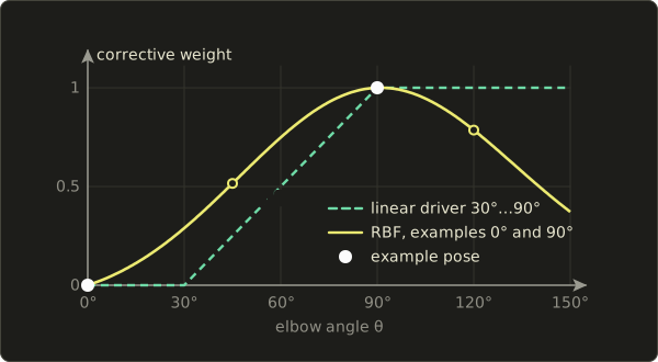
The RBF curve is smooth and passes through both examples, but notice what happens beyond 90°: Gaussian bumps fade with distance, so the correction falls back towards 0 as the elbow bends further, which is usually wrong.
That's the classic trap of RBF interpolation: outside the examples it returns to zero.
Rigs avoid it by sculpting another example at the extreme pose (say 140°), or by adding a linear term to the interpolant.
The same machinery works in many dimensions (all three shoulder angles, or a quaternion distance) and with whole vertex deltas instead of a weight; PSD solvers and RBF nodes are standard tools in DCC rigging at the time of writing.
Delta mush
Delta mush (デルタマッシュ), developed at Rhythm & Hues and presented by Mancewicz and colleagues at DigiPro 2014, cleans up a deformation automatically:
- In the bind pose, smooth the mesh (a few iterations of moving each vertex towards the average of its neighbors, ), and store each vertex's delta from its smoothed position, expressed in a local frame of the smoothed surface (tangent, bitangent, normal).
- At runtime, deform the mesh with any cheap skinning, even rigid binding, smooth the deformed mesh the same way, and add the stored deltas back, rotated into the local frames of the smoothed deformed surface.
The smoothing removes the kinks and collapses of the crude skinning; the deltas put the modeled detail (wrinkles, buttons, muscles) back: a stored delta of 0.3 along the normal, on a smoothed surface point at whose frame has turned by 30°, lands at .
The smoothing costs time every frame, so games often use delta mush offline instead, to bake better LBS weights.
25.4 Blending animation in depth
Chapter 14, section 14.8 listed blending, cross-fades, state machines and blend trees.
What a pose is, and how to blend it
A pose is one local transform per joint, usually stored as translation, rotation quaternion and scale (TRS), relative to the parent.
Blending two poses with the weight is done per joint, in local space:
- translations and scales: linear interpolation;
- rotations: nlerp (normalized lerp, with the sign check) or slerp; most engines use nlerp, because blend weights change every frame anyway and nlerp is cheaper and commutative for many inputs (a weighted sum of several quaternions, then one normalization).
In local space each joint blends only its own rotation, and FK afterwards builds a valid skeleton with the bone lengths intact; blended world matrices would shrink (section 25.1).
1D blend spaces and synchronization
A blend space (ブレンドスペース) places clips at points of a parameter space, and the current parameter value picks the weights.
In 1D, along speed: idle at 0 m/s, walk at 1.5 m/s, run at 4.5 m/s.
At 2.0 m/s, between walk and run:
But a walk cycle lasts 1.2 s and a run cycle 0.8 s; blended frame by frame, the feet would soon be out of step (left foot down in one clip, right foot in the other).
The fix is synchronization (同期) by normalized time (phase): both clips play the same fraction of their cycle, and the blended cycle lasts
so the walk plays at times its speed and the run at times.
Clips are marked with sync markers (foot-down events) so the phases line up even when the clips don't start on the same foot.
A detail that bites: the root speed is not exactly 2.0 now.
The stride per cycle is m for the walk and m for the run; blended, m per 1.1333 s, which is 1.853 m/s.
Either the weight is solved for the exact speed ( here), or the playback rate is raised by , or the stride is adjusted with IK (stride warping).
2D blend spaces with triangles
Locomotion depends on two numbers, the velocity sideways and forward in the character's frame.
A 2D blend space scatters clips over that plane: idle at the center, walks at 1.5 m/s and runs at 4.5 m/s in four directions.
To blend at any point, the samples are triangulated (for example with a Delaunay triangulation), and the query point gets the barycentric coordinates (重心座標) of its triangle as weights, exactly the edge-function areas of chapter 6, section 6.9.
Unreal Engine's blend spaces, for example, use triangulation by default at the time of writing.
Worked example. The query (forward at 2.5 m/s, drifting right at 1.0 m/s) lies in the triangle run F , walk F , run R .
The triangle's area is .
Each weight is the area of the small triangle opposite its vertex, divided by 6.75:
- run F: triangle , walk F, run R, area 3.0, weight ;
- walk F: triangle run F, , run R, area 2.25, weight 0.333;
- run R: triangle run F, walk F, , area 1.5, weight 0.222.
Check: , and the weights add up to 1.
Only three clips are evaluated, and the weights change continuously from one triangle to the next.
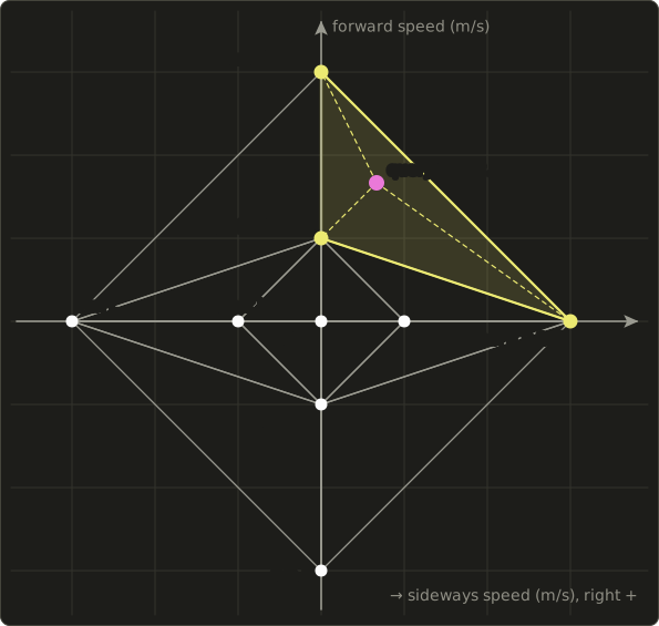
Thin triangles make weights change abruptly, so animators add samples (diagonal walks) where needed.
Additive animation
An additive animation (加算アニメーション) stores a difference from a reference pose instead of a pose: breathing, a flinch, a recoil, leaning into a turn.
For each joint,
where is no rotation, so the weight scales the difference (translations simply add the weighted difference).
Worked example. A flinch bends a spine joint 12° forward about x relative to its reference.
Played with the weight 0.5 on top of a run whose spine is at 20° about x, the result is about x.
Because the difference adds on top of whatever plays underneath, one flinch works on idle, walk and run alike; with several additive layers the order matters, because rotations about different axes don't commute.
Layered and masked blending
Layered blending (レイヤーブレンド) plays different animations on different parts of the body: the legs run while the upper body aims or reloads.
A bone mask (ボーンマスク) gives each joint a weight for the upper layer, often ramped up the spine so the twist is spread out: for example 0.25, 0.5 and 0.75 on three spine joints and 1 from the chest up.
A spine joint with the mask 0.5, at 0° in the run and 40° in the aim pose, gets slerp at 0.5: 20°.
Root motion
The root (ルート) joint of chapter 13 carries the character's motion through the world.
With root motion (ルートモーション) the clip's root displacement is extracted each frame and applied to the character's movement component, so the feet stay planted exactly as captured.
Worked example. The walk clip moves its root 1.8 m forward per 1.2 s cycle, 1.5 m/s; at 60 fps that's m per frame along the clip's forward axis .
The character faces 30° about y, so the displacement in the world is m.
The alternative is in-place animation moved by gameplay code; when the two disagree, the feet slide: code at 2.0 m/s with a walk animated at 1.5 m/s slides 0.5 m every second, unless the playback rate (×1.33) or the stride is adjusted.
Games often use root motion for attacks and climbing, where the exact path matters, and code-driven motion for responsive running.
Transitions: cross-fade vs inertialization
A cross-fade (クロスフェード) from clip A to clip B over 0.2 to 0.3 s evaluates both clips during the whole transition and blends them.
That doubles the cost while it lasts, and the blend can show artifacts of its own (both clips' foot contacts mixed).
Inertialization (慣性化) switches to the new clip immediately and hides the jump with an offset that decays to zero.
David Bollo described it for Gears of War 4 (2016) in talks at SIGGRAPH 2017 and GDC 2018.
At the switch, for each joint (and each channel), record the offset and its rate of change ; then add to the new clip an offset that starts at with velocity and reaches 0 with zero velocity and acceleration after the blend time .
Six conditions call for a polynomial of degree five; with the normalized time , and zero starting acceleration,
If points away from zero (the offset is still growing), it's set to 0 first, so the curve doesn't overshoot.
Bollo's version also chooses a starting acceleration and can shorten , both to prevent overshoot; keeping the acceleration at zero makes the numbers simpler here.
With this is , the quintic "smootherstep" relative of chapter 13's smoothstep.
Worked example. At the switch, an elbow is at 30° and moving at −45°/s in the old clip, and at 10° moving at +15°/s in the new one.
The offset is , its velocity /s (already shrinking, so it's kept), s, :
Check: .
At s (): , so the elbow shows .
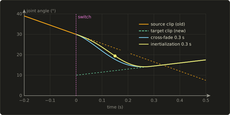
The inertialized curve leaves the old motion with exactly its velocity and lands on the new clip smoothly, and only one clip is evaluated.
For rotations the offset is a quaternion (the rotation from the new pose to the old one), decayed through its axis–angle form.
Unreal Engine, for example, has an inertialization node at the time of writing, and many games now use it for most transitions; it is also what makes motion matching (section 25.5) practical.
State machines, revisited
The state machines of chapter 14 organize all this: each state holds a blend space or blend tree, each transition a condition and a blend method, and big graphs nest sub-state machines.
Their weakness is scale: hundreds of clips need thousands of hand-tuned transitions, the problem motion matching attacks.
25.5 Motion matching
From motion graphs to motion matching
The motion graphs of chapter 13, section 13.9 (Kovar, Gleicher and Pighin, 2002) precompute where one clip can jump into another.
Motion matching (モーションマッチング) drops the precomputation: it keeps a large database of unedited motion capture (minutes of a performer walking, turning, starting and stopping in every combination) and, every few frames at runtime, searches it for the frame that best continues the current pose towards what the player wants.
Simon Clavet of Ubisoft Montreal presented it at GDC 2016 ("Motion Matching and The Road to Next-Gen Animation"), and it shipped in For Honor; since then many games and engines have adopted it.
Features
Each frame of the database gets a feature vector (特徴ベクトル) describing what matters for choosing it, in the character's local frame:
- trajectory features: where the root will be (and which way it will face) a little into the future, for example at 0.33, 0.67 and 1.0 s;
- pose features: positions and velocities of a few key joints, typically the feet and the hips, so the next frame continues the current motion without a jump.
At runtime the query is built the same way: the pose features from the character's current pose, the trajectory features from the player's stick input, predicted forward (often with a spring like those of chapter 14).
Features in different units (meters, meters per second) must be made comparable: each one is normalized by subtracting its mean over the database and dividing by its standard deviation, and then weighted to set priorities (more weight on the trajectory for responsiveness, more on the pose for smoothness).
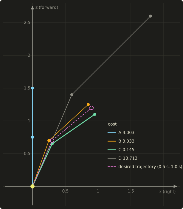
Search: a worked example
A small example with six numbers per frame: the root's future position at 0.5 s and at 1.0 s, and the forward offsets of the left and right foot.
Standard deviations: 0.5 m for the trajectory numbers, 0.2 m for the feet; all weights 1.
The player pushes the stick forward and to the right, and the current pose has the left foot ahead:
Four candidate frames:
| frame | traj. 0.5 s | traj. 1.0 s | feet | trajectory cost | pose cost | total |
|---|---|---|---|---|---|---|
| A: walk straight | (0, 0.75) | (0, 1.5) | (0.12, −0.12) | 3.970 | 0.033 | 4.003 |
| B: walk turning right, other foot | (0.25, 0.7) | (0.85, 1.25) | (−0.10, 0.14) | 0.030 | 3.003 | 3.033 |
| C: walk turning right | (0.3, 0.65) | (0.95, 1.1) | (0.18, −0.05) | 0.060 | 0.085 | 0.145 |
| D: run turning right | (0.6, 1.4) | (1.8, 2.6) | (0.2, −0.2) | 13.400 | 0.313 | 13.713 |
Each cost is the sum of squared normalized differences.
For C: the trajectory differences divided by 0.5 are , squared and summed 0.06; the foot differences divided by 0.2 are , giving .
For B the trajectory is even closer (0.03), but its feet are in the opposite phase: .
Jumping to B would swap the feet in one frame; the pose features prevent that.
C wins, and the character transitions to it, usually with inertialization.
Cost and speed
Real feature vectors have 20 to 30 numbers.
Thirty minutes of capture at 30 frames per second is frames; with 27 floats each, a brute-force search touches million numbers (5.8 MB), several times per second, per character.
That's affordable for the player but not for a crowd, so implementations add acceleration structures (k-d trees, bounding-box hierarchies over the features), search only every 0.1 s or so, and skip the search while the current continuation is good enough.
The capture must cover every motion the player can ask for, and tags exclude frames that don't fit the situation.
Learned motion matching and learned controllers
Learned motion matching (Holden, Kanoun, Perepichka and Popa, SIGGRAPH 2020) replaces the database with small neural networks that do the same job: one predicts the next features (the "stepper"), one does the search's work (the "projector"), and one rebuilds the full pose from the features (the "decompressor"), at a fraction of the memory.
Earlier, phase-functioned neural networks (Holden, Komura and Saito, SIGGRAPH 2017) generated locomotion directly from the user's input and the terrain.
Controllers trained with reinforcement learning can also drive simulated characters with joint torques to imitate captured clips (for example DeepMimic, Peng and colleagues, 2018), physically valid motion that reacts to pushes.
Chapter 29 covers neural networks in rendering.
25.6 Full-body inverse kinematics
Chapter 13 solved IK analytically for two links and iteratively with CCD, and showed the Jacobian.
Here are the methods used for longer chains and whole bodies.
FABRIK
FABRIK (Forward And Backward Reaching Inverse Kinematics; Aristidou and Lasenby, Graphical Models, 2011) works on joint positions, not angles.
It keeps the bone lengths by placing each joint on the line towards its neighbor, at the right distance, in two passes:
- Reachability: if the target is farther from the root than the sum of the bone lengths, stretch the chain straight towards it and stop.
- Backward pass: put the end effector on the target; then, from the end towards the root, move each joint onto the line from its (already moved) child to its current position, at the bone length from the child. The root ends up displaced.
- Forward pass: put the root back where it belongs; then, from the root towards the end, move each joint onto the line from its (already moved) parent to its current position, at the bone length.
- Repeat until the end effector is close enough to the target.
Worked example on chapter 13's arm: , , straight along x (joints at , , ), target , at the distance : reachable.
- Backward: the hand goes to . The elbow moves towards its old position : the direction has length , so the elbow goes to . The root would follow to , 0.146 away from where it must be.
- Forward: the root is put back at . The elbow goes towards , whose length is 2.854: . The hand goes from there towards : the direction has length 1.994, so the hand lands at .
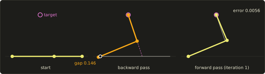
After one iteration the error is 0.0056, after two below 0.0001; CCD needed four sweeps to reach 0.012 on the same problem (chapter 13, section 13.7).
FABRIK's moves are cheap (one normalization per joint, no trigonometry), the bending spreads over the whole chain, and several end effectors (two hands on a rifle) are handled by running the passes per branch and averaging at shared joints.
Angles are read off the final positions: , against the exact 22.62°.
Jacobian methods
The Jacobian of chapter 13 links small joint changes to small end-effector moves, .
To move the effector by the error , there are three classic choices (Samuel Buss's 2004 notes "Introduction to Inverse Kinematics with Jacobian Transpose, Pseudoinverse and Damped Least Squares methods" are the standard tutorial):
- Jacobian transpose (ヤコビ行列の転置法): . No inversion at all; is the direction in which the error falls fastest, and a good step size is .
- Pseudo-inverse (擬似逆行列): , with for a chain with more joints than target coordinates (the smallest joint change that achieves in the linear model); for a square it's simply .
- Damped least squares (DLS, 減衰最小二乗法; Wampler and, independently, Nakamura and Hanafusa, 1986): . The damping trades accuracy for stability: it minimizes , so it never asks for huge joint changes.
Worked example. Chapter 13's FK pose, , , hand at , with
The target is , so , a distance of 0.717.
- Transpose: and , so rad .
- Pseudo-inverse (here ): .
- DLS with : .
Running FK with the new angles, the hand misses the target by 0.035, 0.070 and 0.041.
The pseudo-inverse step is exact for the linear model (it predicts exactly), but the arm moves on arcs, not straight lines, so every method needs a few more iterations; with small errors near the end, all three converge.
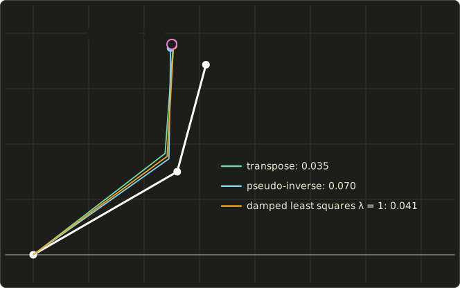
The difference shows near a singular pose (特異姿勢).
Bend the elbow only 5° (, hand at , ) and ask for a hand 0.3 further along x, just out of reach.
The inverse answers with : the arm whips around and the hand lands at .
DLS with answers , a small, harmless step.
That's why solvers damp, and why is often raised automatically as gets small.
Joint limits and other constraints
Iterative solvers enforce the joint limits (可動域) after every step: clamp a hinge angle (a step that asks a knee for 160° gets 150°), project a ball joint's bone back into its allowed cone, and in FABRIK move each joint back into its allowed region relative to its parent during the pass.
A hinge also needs its bending plane: FABRIK alone happily bends a knee backwards if that's closer, which is what the pole vector of chapter 13 or a "mirror into the correct half-plane" rule fixes (the practical assignment shows it).
Foot placement
Animations are captured on flat floors.
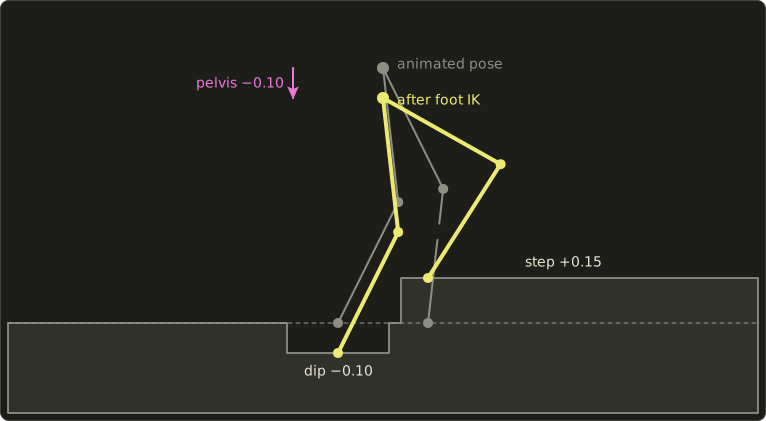
On stairs and slopes, foot IK (フットIK) keeps the feet on the real ground:
- Cast a ray down from each foot's animated position to find the ground height (and normal).
- If a foot must go down (a hole, a lower step), the leg can't reach while the pelvis stays at its animated height, so lower the pelvis by the largest downward offset.
- Solve each leg as a two-bone IK chain (chapter 13's law of cosines) from the lowered hip to its ground point, with a pole vector so the knee points forward.
- Rotate each foot to match the ground normal, and smooth all offsets over time so steps don't pop.
Worked example. Thigh and shin are 0.45 m each.
In the animation the hip is at and the feet at , at the distance ; the knee bend is .
The ground under the back foot has a dip of , and under the front foot a step of .
Lower the pelvis by 0.10 to .
The back foot's target is again 0.863 away, so its knee keeps 32.9°.
The front foot's target is away: , a knee bend of 93.2°.
Look-at
A head that turns towards a point of interest is a small IK problem of its own.
The rotation from the head's forward direction to the target direction has the axis (normalized) and the angle , an axis–angle rotation (Linear Algebra chapter 13, section 13.2) built from a cross and a dot product.
With and a target 60° to the side, : , so the axis is , the angle , and .
Turning only the head looks robotic, so the rotation is distributed, for example 20 % to the spine, 30 % to the neck and 50 % to the head (12°, 18°, 30°, each a slerp from the identity), and clamped to a comfortable cone, beyond which the body should turn instead.
A full-body solver combines such goals (hands on a ledge, feet on the ground, the head on a target, the center of mass over the feet) in one FABRIK-like or damped Jacobian solve over the whole skeleton.
Ragdolls and powered ragdolls
A ragdoll (ラグドール, chapter 14) is the skeleton turned into rigid bodies with joint constraints; it falls convincingly but has no will of its own.
Games blend into a ragdoll when a character is knocked down, and back with a get-up clip that matches the ragdoll's final pose.
A powered ragdoll (also active ragdoll, パワードラグドール) adds a motor at each joint that tries to follow the animation.
The simplest motor is a PD controller (PD制御), a spring towards the target angle plus a damper:
Worked example. An elbow with the moment of inertia kg·m², N·m/rad, N·m·s/rad, lags its animated angle by 0.3 rad while turning at 1 rad/s: N·m, an angular acceleration of rad/s².
These gains are no accident: is critical damping, the same as for the spring of chapter 14, section 14.2: the joint reaches its target fast without oscillating.
High gains follow the animation closely, low gains go limp; a hit reaction lowers the gains of the hit limb for a moment, so the physics pushes it and the animation pulls it back.
How a physics engine solves the joint constraints and motors is chapter 26.
Exam points
Beyond the syllabus, but these sharpen two syllabus items of area 5, character animation and real-time animation (chapters 13 and 14):
- LBS blends matrices, and a weighted sum of rotations is a rotation times a shrink (0.707 at 90°, 0 at 180°): thin bends, candy wrapper. DQS blends rigid transforms as dual quaternions with the same weights, so every vertex moves rigidly: no collapse, but a slight bulge at bends and a flip past 180° of twist.
- The skinning matrix is : the identity in the bind pose.
- Blend in local space, per joint, with slerp or nlerp; 2D blend spaces use barycentric weights of three samples; synchronized clips share a normalized phase.
- Cross-fade evaluates two clips; inertialization evaluates one and decays the offset.
- IK: FABRIK moves positions along lines; Jacobian methods move angles (transpose, pseudo-inverse, damped least squares, the last one stable near singular poses).
25.7 Facial animation in depth
FACS-based rigs and combination shapes
Chapter 13 introduced the Facial Action Coding System (FACS) and its action units (アクションユニット, AU), and FACS-based rigs with roughly one blend shape per AU.
Real faces don't add up linearly, though: a smile (AU12) with the jaw dropped (AU26) stretches the lips differently than the two shapes summed.
So rigs add combination shapes (コンビネーションシェイプ), sculpted corrections for pairs or triples of AUs, whose weight is the product of the weights involved.
With AU12 at 0.8 and AU26 at 0.5, the combination shape gets : zero when either is off, full when both are full.
A film-quality face rig can have hundreds of base and combination shapes, plus correctives for the eyelids sliding over the eyeball and the lips sticking together.
Solving blend shape weights from capture
Performance capture records the face as moving points: markers, or features tracked in video, or a dense reconstructed mesh.
To drive a rig, the capture must be turned into blend shape weights: blend shape solving (ブレンドシェイプのソルブ).
Stack the displacements of the tracked points from the neutral face into a vector , and put each shape's displacements of the same points into a column of a matrix ; then find the weights that reproduce best in the least squares sense:
(the normal equations), usually with the extra conditions and a small penalty that keeps the weights sparse, because a face rig has more shapes than the capture can tell apart.
Worked example with two shapes and three measured numbers: the mouth corner's height, the mouth corner's sideways position and the chin's height.
Smile: ; jaw drop: ; measured .
With the determinant ,
The rebuilt displacements miss the measurement by only 0.014: the capture was a 70 % smile with the jaw 60 % open, plus a little noise that no combination of the shapes can explain, which is exactly what least squares throws away.
At the time of writing, consumer devices do this solve in real time: Apple's ARKit face tracking, for example, outputs named coefficients from 0 (neutral) to 1 (maximum), such as jawOpen and eyeBlinkLeft, ready to drive a rig with matching shapes.
Performance capture
In film and AAA games, performance capture (パフォーマンスキャプチャ) records body, face and voice together, the face with a head-mounted camera.
The footage is tracked, solved onto the actor's own digital double first, retargeted to the character through shared AU names or learned mappings, and polished by animators (eyes, lip contacts for p, b and m).
25.8 Crowds and animation compression
Crowd animation LOD
Chapter 14 introduced crowds and animation LOD.
A typical tier list for a stadium or a battle:
- near: full skeleton, blending, IK;
- middle: fewer bones, updates at 15 to 30 Hz, no IK;
- far: no skeleton: vertex animation textures (VAT, 頂点アニメーションテクスチャ) store the skinned vertex positions of each frame in a texture row, read by the vertex shader by vertex index and time;
- farthest: impostors, the billboards of chapter 12 with a flipbook of animation frames.
A VAT for a 2,000-vertex character and a 60-frame cycle, with positions as four 16-bit floats (8 bytes), is bytes, under 1 MB, and with GPU instancing thousands of copies play it at different phases for almost nothing.
Animation compression
Raw, a clip stores per joint and frame a translation (3 floats), a rotation (4) and a scale (3): 40 bytes; 60 joints at 30 fps make 2,400 bytes per frame and 4.32 MB per minute.
Animation compression (アニメーション圧縮) works in layers:
- Remove constant tracks. Most joints never scale, and only the root translates. Keeping 60 rotations (16 bytes each) plus one root translation (12 bytes) gives 972 bytes per frame, 2.5 times smaller, with no loss at all.
- Keyframe reduction (キーフレーム削減). Remove keys that interpolation between the remaining keys reproduces within a tolerance. A channel with the samples 0, 1.02, 1.98, 3.01, 4.0 at frames 0 to 4 is within 0.02 of the straight line through the first and last, so with a tolerance of 0.05 only two keys remain. Curve fitting with splines (chapter 8) goes further.
- Quantization (量子化). Store values with fewer bits, inside the range each track actually uses.
The classic trick for rotations is smallest three (最小3成分): a unit quaternion satisfies , so one component can be dropped and rebuilt.
Drop the one with the largest magnitude (2 bits say which), and flip the whole quaternion if it's negative ( and are the same rotation); the other three then lie in , which 10 bits each cover in steps of .
That's 32 bits per rotation instead of 128.
Worked example. , 30° about z.
Drop . The code for is , which decodes to 0.2592; and (0) become code 512, which decodes to 0.0007, because no code sits exactly on 0.
Rebuilt: , and the decoded rotation differs from the original by 0.12°.
With rotations at 4 bytes and the root translation as three 16-bit values, a frame needs bytes, 9.8 times smaller than the raw 2,400.
Errors add up along the chain (0.05° at the hip moves a foot 1 m below by mm), so good compressors measure the error at the ends of the chains and give each track just enough bits.
25.9 Summary
- Skinning matrices are , the identity in the bind pose. LBS averages them, and the average of two rotations is a rotation times : thin bends and candy wrappers.
- Dual quaternions () encode rigid transforms. DQS blends them with the LBS weights (sign-checked) and normalizes, so each vertex moves rigidly: the 90° elbow keeps radius 0.5 (LBS 0.354). It bulges slightly at bends, flips past 180° of twist and doesn't handle scale directly.
- Corrective shapes are driven by joint angles and added before skinning; pose-space deformation interpolates sculpted corrections with RBFs (which fall back to zero away from the examples); delta mush smooths a crude deformation and restores the detail.
- Poses blend per joint in local space; blend spaces interpolate weights (1D with phase sync, 2D barycentric in a triangulation); additive layers add differences, masks limit layers to body parts, root motion moves the character with the clip.
- Inertialization switches clips instantly and decays the offset with a quintic, evaluating one clip instead of two.
- Motion matching searches a motion-capture database for the frame whose normalized, weighted features (future trajectory, foot positions and velocities) best match the query; learned motion matching compresses it into networks.
- FABRIK solves IK with positions in backward and forward passes; Jacobian transpose, pseudo-inverse and damped least squares solve it with angles, DLS staying stable near singular poses; joint limits, foot placement and look-at build on them.
- Powered ragdolls drive physics joints towards the animation with PD controllers (critical damping ).
- Faces: FACS shapes plus combination shapes, with weights solved from capture by bounded least squares.
- Crowds use fewer bones, lower update rates, vertex animation textures and impostors; compression removes constant tracks, reduces keys and quantizes (smallest three: 32 bits per rotation).
25.10 Key terms
| English | 日本語 |
|---|---|
| bind pose, inverse bind matrix | バインドポーズ、逆バインド行列 |
| skinning matrix, matrix palette | スキニング行列、行列パレット |
| linear blend skinning (LBS) | リニアブレンドスキニング |
| dual number | 双対数 |
| dual quaternion | デュアルクォータニオン(双対四元数) |
| dual quaternion skinning (DQS) | デュアルクォータニオンスキニング |
| dual quaternion linear blending (DLB) | デュアルクォータニオン線型ブレンド(DLB) |
| flipping artifact, bulge | 反転アーティファクト、膨らみ |
| twist bone | ツイストボーン |
| corrective blend shape | 補正ブレンドシェイプ |
| pose-space deformation (PSD) | ポーズスペースデフォメーション(PSD) |
| radial basis function (RBF) | 放射基底関数(RBF) |
| delta mush | デルタマッシュ |
| pose | ポーズ |
| blend space | ブレンドスペース |
| synchronization, normalized time | 同期、正規化時間 |
| barycentric coordinates | 重心座標 |
| additive animation | 加算アニメーション |
| layered blending, bone mask | レイヤーブレンド、ボーンマスク |
| root motion | ルートモーション |
| cross-fade | クロスフェード |
| inertialization | 慣性化(イナーシャライゼーション) |
| motion matching | モーションマッチング |
| feature vector | 特徴ベクトル |
| learned motion matching | 学習型モーションマッチング |
| FABRIK | FABRIK |
| Jacobian transpose | ヤコビ行列の転置法 |
| pseudo-inverse | 擬似逆行列 |
| damped least squares (DLS) | 減衰最小二乗法 |
| singular pose | 特異姿勢 |
| joint limit | 可動域 |
| foot IK, foot placement | フットIK、足の接地 |
| look-at | ルックアット |
| ragdoll, powered ragdoll | ラグドール、パワードラグドール(アクティブラグドール) |
| PD controller | PD制御 |
| action unit, combination shape | アクションユニット、コンビネーションシェイプ |
| blend shape solving | ブレンドシェイプのソルブ |
| performance capture | パフォーマンスキャプチャ |
| vertex animation texture (VAT) | 頂点アニメーションテクスチャ(VAT) |
| animation compression | アニメーション圧縮 |
| keyframe reduction | キーフレーム削減 |
| quantization, smallest three | 量子化、最小3成分 |
25.11 Challenges
- ★ The elbow of section 25.2 bends by 60° instead of 90° (bone 1 turns about z around ; the vertex has the weights 0.5 and 0.5). Compute the LBS position and its distance from the elbow, then the DQS position (a rotation by half the bend about the elbow), and check that the LBS distance is .
- ★ In the 2D blend space of section 25.4, compute the weights for the queries and , and check that each set reproduces its query. Then compute the 1D weights for 3.5 m/s between walk (1.5 m/s, cycle 1.2 s) and run (4.5 m/s, cycle 0.8 s) and the length of the synchronized cycle.
- ★★ An inertialization starts with the offset , the offset velocity /s and s. Write , check , and compute . Then redo it with /s, and explain why that velocity is set to 0 first.
- ★★ An arm with and lies straight along x, and the target is . Do one FABRIK iteration by hand (backward and forward pass) and give the remaining error. Compare the elbow with the two analytic solutions of chapter 13's law of cosines: which one does FABRIK approach, and why?
- ★★★ Two bones rotate about the same axis through the same point, by 0 and by . Show that DLB with the weight on the second gives a rotation about that same axis and point, by the angle . Evaluate it for and , compare with slerp, and explain where the bulge of section 25.2 comes from.
Multiple choice
Q1 ★ Which of the following statements about dual quaternion skinning is correct?
| A | It blends the entries of the bones' skinning matrices with the weights, exactly like linear blend skinning but with 8 numbers per bone. |
| B | It needs a different set of skin weights from linear blend skinning, so the weights must be painted again. |
| C | A joint twisted by 180° about the bone's axis collapses the skin onto the bone, just as with linear blend skinning. |
| D | It handles non-uniform scaling of bones directly, because a unit dual quaternion can describe any affine transform. |
| E | It blends the bones' rigid transforms as dual quaternions and normalizes the result, so each vertex is moved by a rigid transform; this avoids the candy-wrapper collapse but can make the skin bulge slightly at bent joints. |
Q2 ★ Which of the following statements about animation blending and motion matching is correct?
| A | In a triangulated 2D blend space, every sample clip contributes to the pose with a nonzero weight. |
| B | Inertialization evaluates both the old and the new clip for the whole length of the transition, like a cross-fade. |
| C | Motion matching needs a hand-built state machine with a transition for every pair of clips. |
| D | Motion matching searches a database of animation frames for the frame whose feature vector, for example future trajectory points and foot positions, is closest to a query built from the current pose and the player's input. |
| E | An additive animation stores absolute joint rotations, so it can only be played on its own. |
Q3 ★★ Which of the following statements about inverse kinematics is correct?
| A | FABRIK computes the joint angles with the Jacobian matrix in every iteration. |
| B | Damped least squares adds to before inverting, which keeps the steps small near singular poses such as a fully stretched arm, at the cost of slower convergence. |
| C | The pseudo-inverse step always leaves a smaller error after one step than the Jacobian transpose step, whatever the target. |
| D | CCD moves all joints of the chain at the same time along the gradient of the error. |
| E | Foot placement raises the pelvis to the height of the highest foot target, so that both legs can reach the ground. |
25.12 Practical assignment
Put a leg on a stair step, skin its knee and smooth the transition, all with ruler, compass, protractor and calculator.
You need graph paper (1 unit = 1 cm), a ruler, a compass, a protractor, a pencil, two colored pens and a calculator.
The leg has a thigh and a shin .
The hip is fixed at , and in the bind pose the leg hangs straight down: knee , ankle .
The character faces , so the knee must bend forward (towards ).
The foot must go onto a step at .
- Reach. Measure and compute the distance from to , and check that it's less than .
- FABRIK by construction, two iterations. Backward pass: put the ankle on , draw the line from to the current knee, and mark the new knee with the compass at 4 from on that line. Forward pass: draw the line from to the new knee, mark the knee at 4 from , then the ankle at 4 from the knee towards . Measure the remaining distance from the ankle to . Repeat once. Use the first pen.
- Joint limit. Look at where your knee ended up. If it points backwards (towards ), reflect it across the line (the knee that the pole vector of chapter 13 would choose). Then compute both analytic knee positions with the law of cosines and compare.
- Skin the knee. A vertex sits on the front of the knee in the bind pose, at , with the weights 0.5 (thigh) and 0.5 (shin). Measure the angles by which the thigh and the shin have turned from pointing straight down. Rigid copy 1: turn the vertex about by the thigh's angle. Rigid copy 2: move it with the shin (turn it about by the shin's angle, then move to the new knee). LBS is the midpoint of the two copies; DQS (with equal weights, both copies agree on where goes) turns the vertex about by the average of the two angles and moves to the new knee. Mark both with the second pen and measure their distances from the knee.
- Inertialize the knee. In the animation that was playing, the knee was bent 20° and holding still; the IK result is your knee bend from step 3. Take , and s, compute the knee bend at , and plot the five points against time.
How to check yourself:
- Step 1: .
- Step 2: every bone you drew must measure exactly 4. The error after the first iteration is about 0.31 and after the second about 0.03, so it shrinks roughly tenfold per iteration. Starting from the straight leg, FABRIK bends this knee backwards, to about .
- Step 3: , a knee bend of 75.5°; the two analytic knees are at about and . Your reflected knee must be close to the first one, and each analytic knee must be 4 from and 4 from .
- Step 4: the thigh turns by about 56.2° and the shin by about −19.3° (a difference of 75.5°, the knee bend). The DQS vertex must be 0.5 from the knee, near ; the LBS vertex about from it, near .
- Step 5: the factors are 1, 0.896, 0.5, 0.104 and 0, so the knee goes 20°, 25.8°, 47.8°, 69.8°, 75.5°: exactly halfway at , with flat starts and ends, and never beyond 75.5°.
コメント(0)
まだコメントはありません。
ログインするとコメント出来ます。