15. Image Processing
So far almost everything in this series went from a model to an image.
This chapter is about the step after that: image processing (画像処理), which takes an image and makes another image from it.
In chapter 2 (section 2.11) we sorted the fields by what goes in and what comes out, and image processing was the "image → image" one.
Why does a CG person need it?
Because no rendered frame reaches the screen untouched: a game computes light values far above 1 and tone mapping squeezes them into the display's range, then it blurs, sharpens and color-grades every frame.
Compositors warp, blend and retouch, and textures are made from photos that were straightened and cleaned.
For the exam, this chapter covers all six items of syllabus area 6: representing digital images (ディジタル画像の表現), generating and drawing 2D images (2次元画像の生成と描画), per-pixel tone and color conversion (画素ごとの濃淡変換と色変換), region-based conversion, i.e. spatial filtering (領域に基づく画像変換(空間フィルタリング)), geometric transformation of images (画像の幾何学的変換) and image editing (画像の編集).
It builds on chapter 2, the color spaces, gamma and luminance of chapter 3, the 2D transforms of chapter 4, the rasterization of chapter 6, the Bézier curves of chapter 8, the over operator of chapter 10 and the texture filtering of chapter 11.
Every test image here is generated by a program, and every before/after picture was computed with the formulas in the text.
15.1 Representing digital images
A gray digital image is a function that gives a value for each pixel position: is the column, the row, starting at the top-left corner with y pointing down (section 2.5).
A color image has three such functions, one per channel.
Every operation in this chapter computes a new image from an old one , and it's useful to sort them by how much of the input each output pixel looks at:
- per-pixel (point) operations: depends only on (tone curves, color conversion; sections 15.3 and 15.4);
- local (neighborhood) operations: depends on a small window around (filters; section 15.5);
- geometric operations: takes its value from somewhere else in (rotation, scaling, warping; section 15.6);
- global operations: every output depends on the whole image (histogram equalization, the Fourier transform).
Histograms
The histogram (ヒストグラム) of an image counts how many pixels have each value: = number of pixels with level .
It forgets where the pixels are and keeps only how bright they are: a dark image has its histogram crowded at the left, a low-contrast image has a narrow one, and clipped highlights make a spike at the right end.
We'll use one tiny image for the whole of sections 15.1 and 15.3: 4 × 4 pixels with 8 levels (0 to 7).
Its pixels, row by row, are 1 2 2 5 / 1 2 3 5 / 2 2 4 6 / 1 2 5 5.
Counting gives the histogram:
| level k | 0 | 1 | 2 | 3 | 4 | 5 | 6 | 7 |
|---|---|---|---|---|---|---|---|---|
| h(k) | 0 | 3 | 6 | 1 | 1 | 4 | 1 | 0 |
| cumulative H(k) | 0 | 3 | 9 | 10 | 11 | 15 | 16 | 16 |
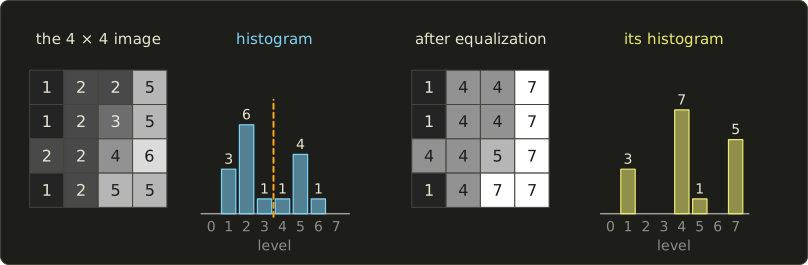
The histogram has two humps, a dark one around level 2 and a bright one around level 5: a bimodal histogram, typical for an object on a background.
The last row is the cumulative histogram (累積ヒストグラム) , the number of pixels at level or darker; it always ends at the pixel count .
Dividing by turns both into fractions, which section 15.3 needs.
Image statistics
Two numbers summarize the histogram.
The mean (平均) is the average brightness and the variance (分散) measures the spread around it, so it is a simple measure of contrast:
For the tiny image: , so .
The squared distances weighted by the counts are , so and the standard deviation (標準偏差) is .
Binary images and neighborhoods
A binary image (二値画像) has only two values, 0 and 1 (background and object).
Binary images come out of thresholding (section 15.3) and are used as masks and for shape analysis.
Working on them needs a definition of which pixels are neighbors: the 4-neighborhood (4近傍) is the pixels to the left, right, above and below; the 8-neighborhood (8近傍) adds the four diagonal ones.
A connected component (連結成分) is a set of object pixels connected through neighbors, and labeling (ラベリング) numbers the components, which is how a program counts objects.
The choice matters: two object pixels that touch only at a corner form one component with 8-connectivity and two components with 4-connectivity.
Color spaces for processing
Which of chapter 3's color spaces is used for what:
- sRGB (gamma-encoded): what files store and most editors operate on; sums and averages of its values are physically wrong (section 3.7).
- Linear RGB: for anything that models light: blurring, resizing, exposure, tone mapping.
- YCbCr (section 3.6): lets a filter treat only the brightness Y (sharpening, denoising).
- HSV / HSL (section 3.5): hue and saturation changes, color-based selection.
- CIELAB: roughly perceptually uniform, for "how different do two colors look".
HDR images
As the HDR teaser of section 2.10 said, a real scene can be far brighter than "as bright as the screen".
The dynamic range (ダイナミックレンジ) is the ratio of the brightest to the darkest value that matters, and photographers count it in stops, factors of two: .
The room scene used later in section 15.4 has luminances from 0.0166 (the floor in shadow) to 282 (the sun in the window): a ratio of about 17,000, or stops.
An 8-bit image can't hold both the shadows and the window.
A high dynamic range image (ハイダイナミックレンジ画像, HDR画像) stores linear light values as floating-point numbers, so that 0.0166 and 282 are both kept with the same relative precision.
Two formats are worth knowing:
- OpenEXR (.exr), developed at Industrial Light & Magic and now the film industry's standard: per channel either 32-bit floats or 16-bit half floats (1 sign bit, 5 exponent bits, 10 mantissa bits). A half covers values up to 65,504 with a relative step of , about three decimal digits everywhere, and allows any number of channels.
- Radiance HDR (.hdr, from Greg Ward's Radiance renderer) with the RGBE encoding: 4 bytes per pixel, an 8-bit mantissa per color channel plus one shared exponent E. The value of a channel is .
Worked example: RGBE.
Encode the linear color .
The largest channel is , so the exponent is 3 and the stored byte is .
Each channel is scaled so that the largest one fills the 8-bit mantissa: the factor is , and , , .
Decoding: , , .
The bright channels come back exactly, the dim one lost 6%: one shared exponent is cheap (4 bytes instead of 12) but gives the darker channels of a strongly colored pixel less precision.
HDR images come from renderers, from merging photos taken at different exposures (chapter 16), and serve as the light probes of chapter 12 (section 12.13); showing one on a screen needs tone mapping (section 15.4).
Image pyramids
Many algorithms want the same image at several scales.
A multi-resolution (多重解像度) representation stacks the image and smaller and smaller copies of it, an image pyramid (画像ピラミッド).
You already know one: the mipmap of section 11.7 is a pyramid built by averaging 2 × 2 blocks, and it costs only a third extra memory.
- A Gaussian pyramid (ガウシアンピラミッド) blurs with a small Gaussian (section 15.5) before each halving, better pre-filtering than the 2 × 2 box.
- A Laplacian pyramid (ラプラシアンピラミッド, Burt and Adelson, 1983) stores at each level the difference between that level and the enlarged next coarser one, plus the smallest level itself; adding them back reconstructs the original exactly.
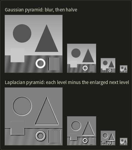
Each Laplacian level is mostly zero (gray) with lines at the edges: one band of frequencies, useful for blending images band by band (panoramas, chapter 16) and coarse-to-fine matching.
15.2 Generating and drawing 2D images
The second syllabus item makes images from shapes: paint programs, vector illustration, user interfaces, PDF viewers and fonts.
Drawing primitives on a raster image
Drawing lines and filling polygons is the rasterization of chapter 6 (Bresenham, section 6.6; circles, 6.7; scanline filling, 6.8), which decides "in or out" per pixel and so produces jaggies.
Anti-aliased drawing
Anti-aliased drawing (アンチエイリアス描画) gives each edge pixel a coverage value: the fraction of the pixel's area inside the shape (area sampling, section 2.7).
The coverage is then used as an alpha value to mix the shape's color with what's already there.
Worked example. A black shape covers 30% of a pixel on a white background.
In linear light the pixel should send out of white, which the sRGB encoding of section 3.7 turns into 0.854, code 218.
Mixing the codes directly would give , visibly darker, which is why naively blended text looks too heavy.
For lines, Xiaolin Wu's algorithm (1991) is the anti-aliased version of Bresenham: at each column it splits the intensity between the two pixels nearest to the exact line, in proportion to the distance; where the line passes at the pixel rows 2 and 3 get 75% and 25%.
2D vector graphics and fill rules
Vector formats such as SVG and PDF (section 2.9) describe a picture as paths (パス): sequences of commands like "move to", "line to", "quadratic or cubic Bézier curve to" (the Bézier curves of section 8.4) and "close".
A path can be stroked (with a width, caps and joins) or filled; for filling, the curves are flattened into short line segments (de Casteljau subdivision) and the polygon is filled.
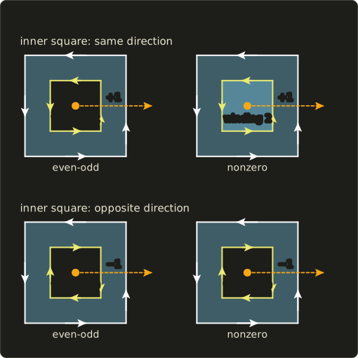
For a path whose parts overlap, "inside" needs a rule, and section 6.8 introduced the two: the even-odd rule (偶奇規則) and the nonzero winding rule (非ゼロ回転数規則).
Both cast a ray from the point to the right; even-odd counts the crossings, nonzero adds +1 for every edge that crosses going up and −1 for every edge going down, the winding number (回転数).
Here is the case that matters most in practice, a square with a square hole:
Worked example.
The outer square runs counter-clockwise, so its right edge goes up: the ray from the center crosses it with +1.
If the inner square also runs counter-clockwise, its right edge adds another +1: winding number 2.
Even-odd sees 2 crossings, an even number, and leaves the center empty; nonzero sees 2 ≠ 0 and fills it.
If the inner square runs clockwise, its right edge goes down and counts −1: winding number , and both rules leave a hole.
A point between the two squares has winding number 1 in both cases and is filled by both rules.
That's why font and icon designers draw holes (the inside of an "o") with the opposite direction to the outline: then the hole comes out right no matter which rule the renderer uses.
Fonts and text rendering
An outline font (アウトラインフォント) stores each glyph as filled paths: TrueType with quadratic Bézier curves, PostScript/CFF (OpenType) with cubic ones (section 8.4).
A bitmap font (ビットマップフォント) stores ready-made pixel images at fixed sizes.
At small sizes a stem 1.4 pixels wide falls on the pixel grid differently in every letter, so hinting (ヒンティング) nudges the outline so that stems and baselines land on whole pixels.
Games often store glyphs as a signed distance field texture, which stays sharp at any scale; you'll draw text in the OpenGL series, chapter 26.
Paint tools and brushes
A paint program's brush is almost always stamping: copies of a small brush image are placed at regular distances along the stroke and blended onto the canvas.
The spacing (as a fraction of the brush diameter) decides whether the stroke looks continuous, and the flow (the opacity of each stamp) decides how fast paint builds up where stamps overlap.
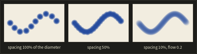
Worked example. A stroke 100 pixels long with a 20-pixel brush and spacing 25% puts a stamp every pixels, so stamps.
With a flow of 0.2, each stamp is blended with the over operator, so a point covered by stamps reaches the opacity : 0.2, 0.36, 0.488, 0.590 for .
Pen pressure usually scales the size or flow of each stamp.
Compositing layers with alpha
Drawing programs combine layers (レイヤー) from bottom to top with the over operator of section 10.12; when both layers can be partly transparent, the full formula is
The division disappears with premultiplied alpha (乗算済みアルファ), , which chapter 14 (section 14.10) introduced together with its other advantages: over becomes the same simple formula for the color and for alpha, .
Worked example. Red with over blue with .
Premultiplied: , .
and .
Dividing by gives the ordinary color .
15.3 Per-pixel tone conversion
A per-pixel (point) operation computes each output value from the input value at the same pixel only: .
Converting gray levels this way is gray-level or tone conversion (濃淡変換); doing it to colors is color conversion (section 15.4).
Tone curves
The function is drawn as a graph from input to output, the tone curve (トーンカーブ).
The diagonal changes nothing; the steeper the curve, the more contrast in that range of values.
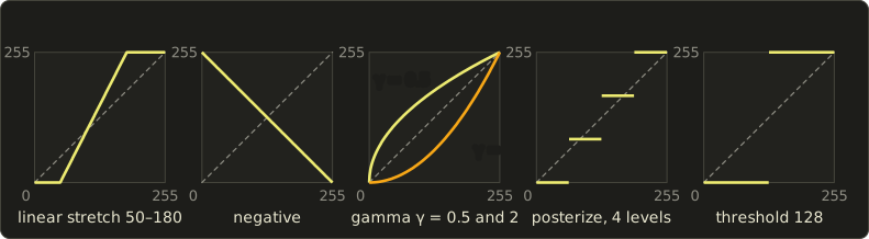
With 8-bit values from 0 to 255, the classic curves and one worked value each:
- Linear stretch (線型の引き伸ばし, contrast stretching): map the occupied range onto the full range, , clipped to 0–255. With , : gives .
- Negative (ネガ, 反転): . 100 becomes 155.
- Gamma (ガンマ変換): . brightens the dark tones, darkens them. With , gives ; with it gives . (This is the same kind of power curve as the display gamma of section 3.7, used here as an editing tool.)
- Posterization (ポスタリゼーション): keep only levels, . With , : , so . Posterization creates the false contours of section 2.8 on purpose.
- Contrast and brightness (コントラスト、明るさ): ; contrast rotates the line around the middle gray, brightness shifts it. With , : gives .
- Threshold: a step from 0 to 255, the binarization below.
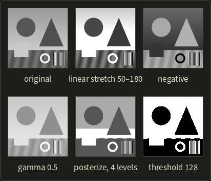
A tone curve maps equal inputs to equal outputs everywhere, so it can't lighten one gray square without lightening every square of that gray; that needs masks or local operations.
Lookup tables
An 8-bit image has only 256 possible input values, so instead of evaluating (maybe a power function) for millions of pixels, a program evaluates it 256 times and stores the results in a lookup table (ルックアップテーブル, LUT).
The conversion of a pixel is then one array access, g = lut[f].
For color, a 3D LUT maps RGB to RGB; a typical grading LUT has entries, interpolated trilinearly, and game engines apply such "looks" as a 3D texture in post-processing.
Binarization and Otsu's method
Binarization (二値化) turns a gray image into a binary one with a threshold (しきい値) : pixels above become 1, the others 0.
A fixed threshold such as 128 works only when you know the brightness in advance.
Otsu's method (大津の方法, Nobuyuki Otsu, 1979; also called the discriminant analysis method, 判別分析法) chooses from the histogram alone.
Splitting the levels at gives two classes, dark () and bright (), with pixel fractions and mean levels .
A good threshold makes the two classes far apart and each one tight; Otsu maximizes the between-class variance
which is the same as minimizing the variance within the classes, because the two always add up to the total variance .
Worked example on the tiny image (with ):
| t | |||||
|---|---|---|---|---|---|
| 1 | 3/16 | 13/16 | 1 | 45/13 ≈ 3.462 | 0.923 |
| 2 | 9/16 | 7/16 | 15/9 ≈ 1.667 | 33/7 ≈ 4.714 | 2.286 |
| 3 | 10/16 | 6/16 | 1.8 | 5 | 2.4 |
| 4 | 11/16 | 5/16 | 2 | 5.2 | 2.2 |
| 5 | 15/16 | 1/16 | 2.8 | 6 | 0.6 |
For : the dark class holds levels 1, 2, 3 with pixels and the sum , so ; the bright class holds levels 4, 5, 6 with pixels and the sum , so .
, the maximum: Otsu's threshold is , the dashed line in the histogram figure.
Check: the variances within the classes are 0.36 (dark) and 0.333 (bright), weighted , and .
(Thresholds 0 and 6 leave one class empty and are skipped.)
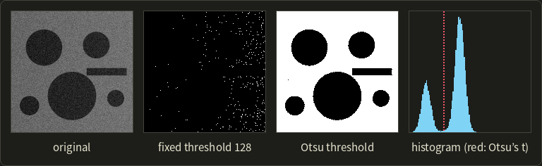
Here the background sits around 107 and the discs around 36, so the fixed threshold 128 calls everything dark, while Otsu finds in the valley.
When the lighting varies across the image, adaptive thresholding computes a threshold per region instead.
Histogram equalization
A low-contrast image uses only part of the available levels.
Histogram equalization (ヒストグラム平坦化, also 均等化) spreads them out by using the cumulative histogram as the tone curve:
with levels and pixels.
A level that 10% of the pixels are darker than goes to 10% of the output range, so crowded parts of the histogram get stretched.
Worked example on the tiny image, , :
| k | 1 | 2 | 3 | 4 | 5 | 6 |
|---|---|---|---|---|---|---|
| H(k) | 3 | 9 | 10 | 11 | 15 | 16 |
| 7 H(k) / 16 | 1.3125 | 3.9375 | 4.375 | 4.8125 | 6.5625 | 7 |
| g(k) | 1 | 4 | 4 | 5 | 7 | 7 |
The image becomes 1 4 4 7 / 1 4 4 7 / 4 4 5 7 / 1 4 7 7, with the histogram (the right half of the first figure in this chapter).
The mean rose from 3 to 4.4375 and the variance from 2.75 to 4.371: more contrast, and the full range 1 to 7 is used.
Three things are worth noticing, and all three are worth being sure about for the exam:
- The result is not flat. Pixels with the same input level always get the same output level, so a tall bar can't be split; equalization only moves bars apart.
- Levels can merge: 2 and 3 both became 4, 5 and 6 both became 7. The number of distinct levels never grows, it can only shrink.
- The curve is monotonic (never decreasing), so the order of brightness is kept: a darker pixel never becomes brighter than a brighter one.
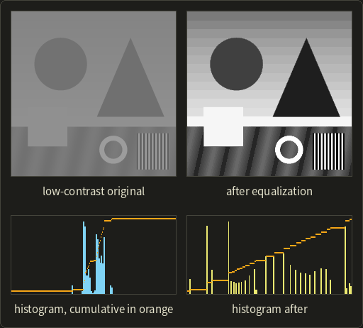
Details appear, but smooth areas (the sky) get stretched into visible bands and noise is amplified.
Some books use so that the darkest occupied level maps to exactly 0; CLAHE equalizes small tiles separately with a limited slope, common in medical imaging.
15.4 Color conversion and tone mapping
Color conversion (色変換) applies a per-pixel function to all three channels at once.
Many of the useful ones are 3 × 3 matrices: with , the matrix–vector product of linalg chapter 6.
All worked examples below use the color , an orange.
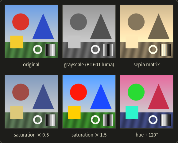
Grayscale
A gray version weights the channels by how bright they look (section 3.6).
Editors usually apply the luma formula to the stored values: with BT.601 weights, .
The physically correct way decodes to linear first, , takes the BT.709 luminance , and encodes it again: 0.5125.
The plain average is the crudest choice: it makes blue as bright as green.
Color matrices: saturation, sepia and white balance
Saturation (彩度) moves a color away from or towards its own gray: per channel.
With : gives gray , gives , and gives .
Because is a linear combination of R, G and B, this whole operation is one 3 × 3 matrix too.
A sepia (セピア) tone, the brown of old photographs, is a matrix whose rows are all "luminance-like" sums with different weights; a commonly used one is
For our orange: , , .
Every color becomes a shade of the same brown; white maps to and must be clipped.
White balance (ホワイトバランス, section 3.8) is the diagonal matrix that scales each channel so that a gray object comes out neutral; it should be applied to linear values.
Hue rotation
Rotating the hue (色相) shifts every color around the color wheel.
The clean way is through HSV (section 3.5): convert, add the angle to H, convert back.
Worked example. has , and .
Add 120°: , in the sector from 120° to 180° where green is the largest channel.
So , , and B rises from the minimum: , giving .
A rotation by exactly 120° just moves the channels around, ; shaders often approximate other angles with a 3 × 3 rotation about the gray axis of RGB space.
Tone mapping HDR images
Now the promise from chapters 2, 3 and 10: showing an HDR image on a screen that goes from 0 to 1.
Tone mapping (トーンマッピング) is a tone curve from scene luminance (0 to "anything") to display values (0 to 1).
The step before it is exposure (露出): multiply the linear values by , so +1 EV doubles the brightness and −2 EV divides it by 4, exactly like opening or closing the camera by a stop (section 2.3).
Doing nothing means clipping, : at exposure 0 the window is pure white, at −5 EV the room is black.
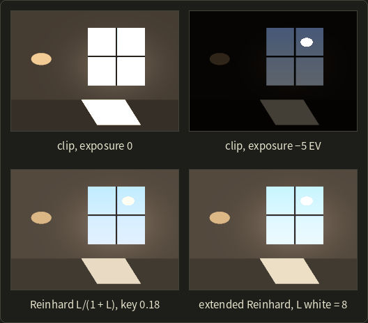
Reinhard's operator (Reinhard and colleagues, 2002) compresses instead of clipping:
Small values pass almost unchanged (), becomes 0.5, becomes 0.8, and even only reaches 0.990: everything fits, nothing clips, and contrast is taken away mostly from the highlights.
The extended version lets the brightest value reach exactly 1:
With : gives and gives .
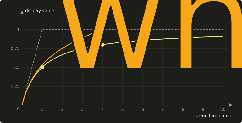
To choose the exposure automatically, Reinhard scales the image so that its log-average luminance (対数平均輝度) lands on a key value (キー値) , usually 0.18 (middle gray):
( is a tiny number that avoids ; the geometric mean keeps the sun from dominating.)
Worked example. Four pixels with luminances 0.01, 0.1, 1 and 10 (ignore ).
.
Scale factor : the luminances become 0.00569, 0.0569, 0.5692 and 5.692.
Reinhard: 0.00566, 0.0539, 0.3627 and 0.8506.
Encoded to sRGB for the screen (section 3.7): 0.067, 0.257, 0.636 and 0.931.
A ratio of 1000:1 (almost 10 stops) now fits on the display, with the darkest pixel still distinguishable from black.
Tone mapping should act on luminance and scale the color with it, , so that hues stay the same.
Games mostly use S-shaped "filmic" curves such as ACES; all of these are global (one curve for the whole image), while local operators adapt to each region like the eye does (Part 2).
In a shader
Real-time renderers draw into a floating-point framebuffer and tone map it in a full-screen pass, whose core looks like this:
// Exposure, then Reinhard on luminance; the result is still linear.
float3 toneMapReinhard(float3 hdr, float exposureEv) {
  float3 c = hdr * exp2(exposureEv);
  float L = dot(c, float3(0.2126, 0.7152, 0.0722));
  float Ld = L / (1.0 + L);
  return saturate(c * (Ld / max(L, 1e-6)));
}
// Exposure, then Reinhard on luminance; the result is still linear.
vec3 toneMapReinhard(vec3 hdr, float exposureEv) {
vec3 c = hdr * exp2(exposureEv);
float L = dot(c, vec3(0.2126, 0.7152, 0.0722));
float Ld = L / (1.0 + L);
return clamp(c * (Ld / max(L, 1e-6)), 0.0, 1.0);
}// Exposure, then Reinhard on luminance; the result is still linear.
float3 toneMapReinhard(float3 hdr, float exposureEv) {
float3 c = hdr * exp2(exposureEv);
float L = dot(c, float3(0.2126, 0.7152, 0.0722));
float Ld = L / (1.0 + L);
return saturate(c * (Ld / max(L, 1e-6)));
}
The final clamp is needed because scaling a saturated color by can push a single channel above 1 even though the luminance is below 1.
The result is then encoded to sRGB, by hand (section 3.10) or by writing to an sRGB framebuffer.
You'll build exactly this pass in the OpenGL series, chapter 21.
Exam points
- Point operations: ; a tone curve cannot tell two pixels of the same value apart. Linear stretch , negative , gamma ( brightens), posterization, threshold.
- A LUT precomputes for every possible input value (256 entries for 8 bits).
- Otsu's method picks the threshold that maximizes the between-class variance (equivalently minimizes the within-class variance).
- Histogram equalization uses the normalized cumulative histogram as the tone curve; the result is not perfectly flat, levels can merge but never split, and brightness order is kept.
- Grayscale: weighted sum (BT.601 0.299/0.587/0.114 for luma, BT.709 0.2126/0.7152/0.0722 for linear luminance), not the plain average.
- HDR images store linear floating-point values (OpenEXR half/float, Radiance RGBE with a shared exponent); tone mapping compresses them to 0–1, e.g. Reinhard after scaling by key/log-average.
15.5 Spatial filtering
A spatial filter (空間フィルタ) computes each output pixel from a neighborhood of the input pixel: this is the region-based conversion of the syllabus, spatial filtering (空間フィルタリング).
Most filters are linear and are written as a small table of weights.
Convolution
The weights form a kernel (カーネル), also called the filter mask or filter coefficients, usually 3 × 3 or 5 × 5 with the center at .
The output is the weighted sum of the neighborhood:
Strictly, this is correlation (相関); convolution (畳み込み) in the mathematical sense uses , which is the same as correlation with the kernel rotated by 180°.
For symmetric kernels the two are identical, for the edge kernels below flipping only changes the sign, and texts usually call both "convolution".
Our worked grid for this whole section is a 5 × 5 image with a vertical edge (10 on the left, 90 on the right) and one bright noise pixel of 250:
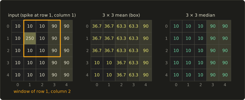
Worked example: the 3 × 3 mean filter. For row 1, column 2, the window (orange) holds 10 10 90 / 250 10 90 / 10 10 90.
The sum is 570, and .
The pixel was 10 and became 63.3: averaging spreads the spike into a 3 × 3 blotch and smears the edge over two columns (36.7, 63.3 in the bottom rows instead of a jump from 10 to 90).
Border handling
At the image border part of the window falls outside the image, and something must be assumed there: zero padding (outside = 0), clamp (repeat the edge pixel), mirror or wrap (periodic), the wrap modes of section 11.6 again, or simply a smaller output.
In the grid, the top-right pixel (row 0, column 4) is 90 and all its neighbors are 90 too.
With clamping its mean is 90, but with zero padding five of the nine window values are 0 and the mean is : a dark frame appears around the image.
The figure above uses clamping, which is the usual choice.
Smoothing: box and Gaussian filters
Smoothing (平滑化) filters average neighboring pixels to reduce noise, at the cost of blurring.
The mean filter (平均値フィルタ, also box filter or moving average) gives all pixels the weight .
The Gaussian filter (ガウシアンフィルタ) weights them by the bell curve , so near pixels count more; sets the blur radius, and a kernel of about holds almost all the weight.
The smallest integer approximation is
At the spike (row 1, column 1): , compared with 36.7 from the mean filter.
The Gaussian keeps more of the center, and it has no sharp cutoff, which matters in the frequency domain below.
Separability
The Gaussian kernel above is the outer product of with itself: the filter is separable (分離可能).
Filtering the rows with and then the columns with the same kernel gives exactly the 2D result.
Worked check at the spike: the horizontal pass gives, in column 1, for row 0, for row 1 and for row 2.
The vertical pass: , the same as before.
The payoff is speed: an kernel costs multiplications per pixel, two 1D passes cost : for a 15 × 15 Gaussian, 30 instead of 225.
The median filter
The median filter (メディアンフィルタ) sorts the values and takes the middle one.
In the window of row 1, column 2 the sorted values are 10 10 10 10 10 90 90 90 250: the median is 10, the correct value.
The whole result (the right grid in the figure) is the original image without the spike, and the edge is still a perfect jump from 10 to 90.
One extreme value can never pull the median, and at a straight edge most of the window lies on the pixel's own side; the median is not linear, so it has no kernel.
Which filter for which noise is worth being sure about for the exam:
- Gaussian noise (ガウスノイズ): every pixel is off by a small random amount (sensor noise). Averaging works: Gaussian, box, or the bilateral filter below.
- Salt-and-pepper noise (ごま塩ノイズ): a few pixels are completely wrong, black or white. Averaging smears them; the median removes them.
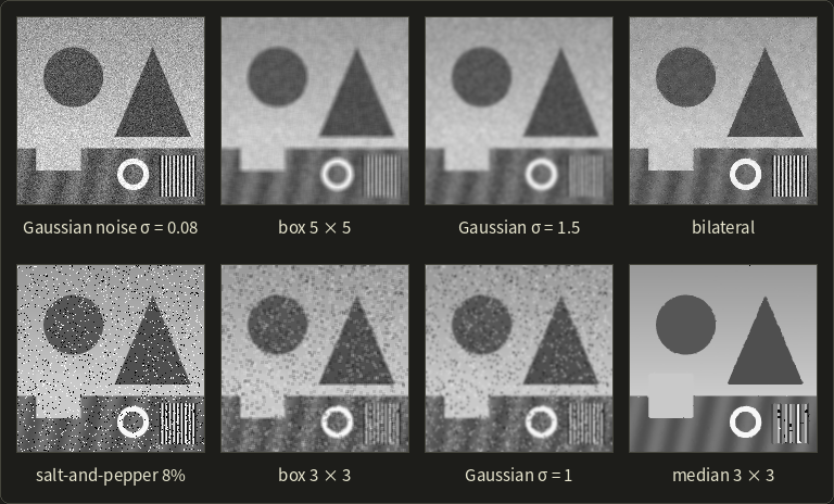
The median removed every speck but also damaged the fine stripes: a 1-pixel stripe is a minority in its window, just like noise.
Edge detection: differences, Prewitt and Sobel
An edge (エッジ) is where the brightness changes quickly, and edge detection (エッジ検出) looks for large values of the derivative.
On pixels the derivative becomes a difference: forward or central .
In 2D the two partial derivatives form the gradient (勾配) ; its length is the edge strength and its direction points across the edge, towards the brighter side.
A plain difference reacts strongly to noise, so practical differential filters (微分フィルタ) take the difference in one direction and smooth in the other.
The Prewitt filter (プリューウィットフィルタ) smooths with equal weights, the Sobel filter (ソーベルフィルタ) with 1 2 1:
The vertical kernels are the transposes; with y pointing down, responds positively when the image gets brighter downwards.
Worked example. A 3 × 3 patch on a diagonal edge, dark at the top left: 10 10 40 / 10 40 90 / 40 90 90.
Sobel x: each row's right value minus left value, weighted 1, 2, 1: .
Sobel y: bottom row minus top row, weighted 1, 2, 1: .
Magnitude (the approximation gives 480), direction : pointing right and down, across the diagonal edge towards the bright corner.
Prewitt on the same patch gives , the same direction with a different scale.
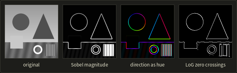
Run Sobel on our 5 × 5 grid and you'll see the downside of derivatives: the spike produces magnitudes of up to 480 all around it, larger than the real edge (320), which is why edge detectors smooth first.
The Canny edge detector (キャニー法, 1986) does exactly that: Gaussian smoothing, Sobel gradient, non-maximum suppression (thin the edges to 1 pixel) and hysteresis thresholding (a strong threshold to start an edge, a weaker one to continue it).
The Laplacian and zero crossings
The second derivative gives another view of an edge.
The Laplacian becomes, with the second difference in both directions, the Laplacian filter (ラプラシアンフィルタ):
It is isotropic (one number, no direction) and even more sensitive to noise than the first derivative.
On the diagonal patch above: 4-neighbor , 8-neighbor .
Where is the edge exactly?
Worked example in 1D: the profile 10 10 10 30 70 90 90 90 (pixels 0 to 7) is a soft edge.
The central differences at pixels 1 to 6 are 0, 10, 30, 30, 10, 0: largest at pixels 3 and 4.
The second differences at pixels 1 to 6 are 0, 20, 20, −20, −20, 0: positive before the edge, negative after it.
The edge is where the second derivative changes sign, the zero crossing (ゼロ交差), here between pixels 3 and 4, exactly between 30 and 70.
Smoothing first gives the LoG filter (Laplacian of Gaussian, Marr and Hildreth, 1980), the fourth picture above.
Sharpening and unsharp masking
Sharpening (鮮鋭化) boosts the detail.
The classic darkroom trick, unsharp masking (アンシャープマスキング), subtracts a blurred copy to get the detail and adds it back with a strength :
Worked example on the profile 10 10 10 30 70 90 90 90 with the blur (clamped borders) and :
| pixel | 0 | 1 | 2 | 3 | 4 | 5 | 6 | 7 |
|---|---|---|---|---|---|---|---|---|
| f | 10 | 10 | 10 | 30 | 70 | 90 | 90 | 90 |
| blur(f) | 10 | 10 | 15 | 35 | 65 | 85 | 90 | 90 |
| f − blur(f) | 0 | 0 | −5 | −5 | 5 | 5 | 0 | 0 |
| g | 10 | 10 | 5 | 25 | 75 | 95 | 90 | 90 |
For example at pixel 3: , so .
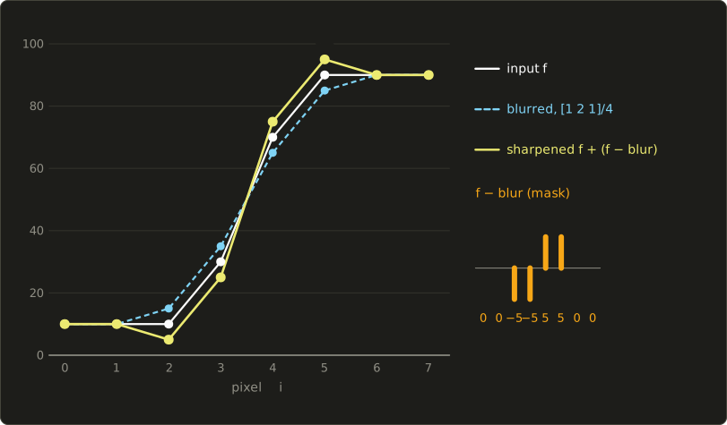
The edge got steeper (25 to 75 instead of 30 to 70), and it got a dark undershoot (5) and a bright overshoot (95) on either side.
Those make the edge look crisper, but with a large they become visible halos:
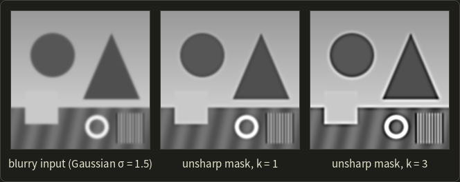
Sharpening and the Laplacian are closely related: with this blur, in 1D, so unsharp masking is "subtract a bit of the Laplacian", (challenge 5).
The bilateral filter
The bilateral filter (バイラテラルフィルタ, Tomasi and Manduchi, 1998) is a Gaussian whose weights are also multiplied by a second Gaussian of the difference in value:
Worked example. With and , at a pixel of value 10 next to an edge to 90: a direct neighbor on the same side gets , a direct neighbor across the edge gets .
Pixels across the edge are effectively ignored.
For a 3 × 3 window 10 10 90 / 10 10 90 / 10 10 90 centered on a 10, the plain Gaussian gives 31.9 and the bilateral gives 10.01.
It smooths without blurring edges; it is nonlinear and slower, and is behind many denoisers and skin-smoothing tools; chapter 16 uses a variant of it for flash/no-flash photography.
Morphology on binary images
Morphology (モルフォロジー) processes the shapes in a binary image with a small structuring element (構造要素), here a 3 × 3 square.
- Dilation (膨張): a pixel becomes 1 if any pixel under the element is 1. Shapes grow by one pixel all around; holes and gaps shrink.
- Erosion (収縮): a pixel stays 1 only if all pixels under the element are 1. Shapes shrink; thin parts and specks vanish.
- Opening (オープニング): erosion, then dilation. Removes specks and thin protrusions smaller than the element, and restores the rest to (almost) its original shape.
- Closing (クロージング): dilation, then erosion. Fills small holes and gaps, and restores the outline.
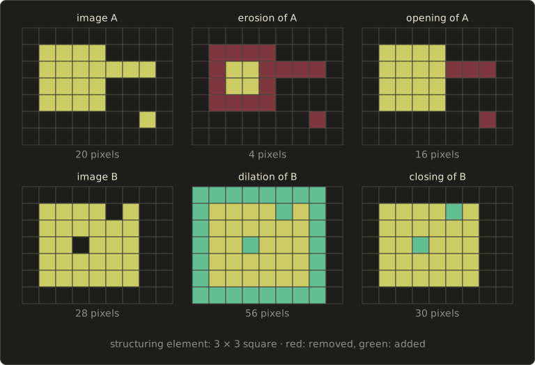
Worked example. Image A is a 4 × 4 block (16 pixels) with a 3-pixel spur and one isolated speck, 20 pixels in all.
Erosion keeps only the pixels whose whole 3 × 3 neighborhood is inside: the inner 2 × 2 of the block, 4 pixels; the spur (1 pixel thick) and the speck vanish.
Dilating those 4 pixels gives back the 4 × 4 block: the opening has 16 pixels, the original without spur and speck.
Image B is a 5 × 6 block with a one-pixel hole and a notch in its top edge, 28 pixels.
Dilation fills both and grows the block to 7 × 8 = 56 pixels; erosion shrinks it back, and the closing is the complete 5 × 6 block, 30 pixels.
Opening and closing clean up thresholded images and masks; on gray images they become local minimum and maximum filters.
The frequency domain
The Fourier transform (フーリエ変換) rewrites an image as a sum of sine waves (stripes) of different frequencies and directions, just like the DCT of JPEG in section 2.10 rewrote 8 × 8 blocks.
Low frequencies are the smooth, large-scale parts; high frequencies are edges, fine texture and noise.
The convolution theorem (畳み込み定理) says that convolving with a kernel in the image is the same as multiplying the spectrum by the kernel's own spectrum, its frequency response.
So a smoothing filter is a low-pass filter (ローパスフィルタ, it keeps low frequencies) and a sharpening or edge filter is a high-pass filter (ハイパスフィルタ).
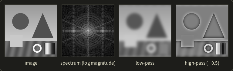
In the spectrum the center is frequency zero and the distance from it is the frequency; the bright lines come from the straight edges.
Worked example. The finest possible pattern is the 1D checkerboard +1, −1, +1, −1, …, at the Nyquist frequency of section 2.6.
A 3-tap box filter at a +1 pixel gives : the pattern survives at a third of its strength, inverted.
The kernel gives : removed completely.
In general their frequency responses are and for from 0 to (radians per pixel), and the box's response goes negative.
Sharp-edged kernels misbehave: the box passes some high frequencies with flipped sign, and an "ideal" low-pass that cuts the spectrum sharply rings next to every edge, while the Gaussian's spectrum is again a smooth Gaussian.
Pre-filtering before downsampling (chapter 2) is exactly a low-pass filter, and deblurring (deconvolution, chapter 16) works in the frequency domain.
C++: a 3 × 3 filter
Here is a general 3 × 3 filter with clamped borders, applied to the 5 × 5 grid with the box kernel and with Sobel:
#include <cmath>
#include <cstdio>

// A gray image of w x h pixels, row 0 first.
struct Image {
  int w, h;
  float *px;
  float at(int x, int y) const { // clamp to the border ("replicate")
    x = x < 0 ? 0 : (x >= w ? w - 1 : x);
    y = y < 0 ? 0 : (y >= h ? h - 1 : y);
    return px[y * w + x];
  }
};

// out(x, y) = sum of k(i, j) * in(x + i, y + j) for i, j in -1..1
// (correlation: the kernel is not flipped).
void filter3x3(const Image &in, const float (&k)[3][3], Image &out) {
  for (int y = 0; y < in.h; ++y) {
    for (int x = 0; x < in.w; ++x) {
      float s = 0;
      for (int j = -1; j <= 1; ++j)
        for (int i = -1; i <= 1; ++i) s += k[j + 1][i + 1] * in.at(x + i, y + j);
      out.px[y * out.w + x] = s;
    }
  }
}

int main() {
  float a[25] = {10, 10, 10, 90, 90, 10, 250, 10, 90, 90, 10, 10, 10, 90, 90,
                 10, 10, 10, 90, 90, 10, 10, 10, 90, 90};
  float b[25], gx[25], gy[25];
  Image in{5, 5, a}, box{5, 5, b}, sx{5, 5, gx}, sy{5, 5, gy};
  const float t = 1 / 9.f;
  const float boxK[3][3] = {{t, t, t}, {t, t, t}, {t, t, t}};
  const float sobelX[3][3] = {{-1, 0, 1}, {-2, 0, 2}, {-1, 0, 1}};
  const float sobelY[3][3] = {{-1, -2, -1}, {0, 0, 0}, {1, 2, 1}};
  filter3x3(in, boxK, box);
  filter3x3(in, sobelX, sx);
  filter3x3(in, sobelY, sy);
  for (int y = 0; y < 5; ++y) {
    printf("box:");
    for (int x = 0; x < 5; ++x) printf(" %6.2f", b[y * 5 + x]);
    printf("   |G|:");
    for (int x = 0; x < 5; ++x) printf(" %4.0f", std::hypot(gx[y * 5 + x], gy[y * 5 + x]));
    printf("\n");
  }
  return 0;
}
box:  36.67  36.67  63.33  63.33  90.00   |G|:  339  480  253  320    0
box:  36.67  36.67  63.33  63.33  90.00   |G|:  480    0  160  320    0
box:  36.67  36.67  63.33  63.33  90.00   |G|:  339  480  253  320    0
box:  10.00  10.00  36.67  63.33  90.00   |G|:    0    0  320  320    0
box:  10.00  10.00  36.67  63.33  90.00   |G|:    0    0  320  320    0
The bottom rows show the clean edge (320); the top rows show a single noise pixel lighting up a ring of "edges" while the spike itself gets 0.
On a GPU the same runs as a post-processing pass; you'll write such kernels in the OpenGL series, chapter 17.
Exam points
- Linear filters are convolutions (correlations) with a kernel; separable kernels (box, Gaussian) can be applied as two 1D passes ( instead of operations).
- Border handling: zero padding darkens the border; clamp, mirror and wrap don't.
- Gaussian noise → averaging (Gaussian, box, bilateral); salt-and-pepper noise → median. The median is nonlinear and keeps edges.
- First derivative: Prewitt, Sobel (difference in one direction, smoothing in the other; gradient magnitude and direction). Second derivative: Laplacian (isotropic, no direction, edges at zero crossings, very noise sensitive).
- Unsharp masking: , steeper edges with overshoot; too strong → halos.
- Dilation grows, erosion shrinks; opening (erosion → dilation) removes small bright parts, closing (dilation → erosion) fills small holes.
- Smoothing = low-pass, edge detection and sharpening = high-pass; convolution in space = multiplication in frequency.
15.6 Geometric transformation of images
Rotating, scaling or warping an image moves pixels instead of changing their values: a geometric transformation (幾何学的変換).
The transform is the math of chapter 4; the new question is where the pixel values come from.
Forward and inverse mapping
The obvious way is forward mapping (順方向マッピング): go through the input pixels, transform each position, and write the value into the output pixel it lands on.
When enlarging, some output pixels are never hit: holes (穴); when shrinking, several input pixels overwrite each other.
Worked example. Enlarging by 1.2 makes times as many output pixels, so at least of them stay empty; in the left picture below (30° rotation, 1.2× enlargement), 10,648 of 34,848 output pixels got no value, exactly that 30.6%.
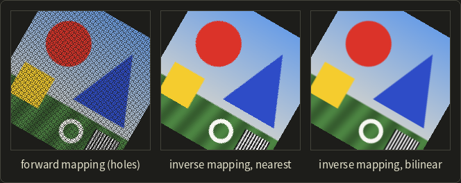
Inverse mapping (逆方向マッピング) turns the loop around: go through the output pixels, apply the inverse transform to find where each one comes from in the input, and read the input there.
The same pair of words, forward and backward (順方向・逆方向), also describes the direction in which rays are followed in ray tracing (section 12.8); the idea is the same: start from what you want to fill (the output pixel, the eye) and look backwards for where it comes from.
Every output pixel gets exactly one value, and since the position in the input is rarely a pixel center, it is interpolated: resampling (再標本化, リサンプリング).
Texture mapping on a GPU (chapter 11) works the same way.
Affine transforms of images
For an affine transform (section 4.4) the inverse is again affine (section 4.3), so the inverse mapping costs the same as the forward one.
Worked example. Rotate an image by about its center (pixel coordinates).
The forward map is , so the inverse is (the inverse of a rotation is its transpose, linalg chapter 10).
For the output pixel : , and
so the value comes from in the input, between the pixels 75 and 76 of row 35.
(With y pointing down on the screen, this positive angle turns the picture clockwise; section 4.1 discussed the flipped axis.)
Resampling: nearest, bilinear and bicubic
The interpolation methods are the ones of section 11.7, now on images:
- Nearest-neighbor interpolation (最近傍補間): take the closest pixel. Fast, keeps hard pixel edges, but enlarged images look blocky and rotated edges get jagged.
- Bilinear interpolation (双線型補間): blend the 4 surrounding pixels linearly in x and in y. Smooth, but blurry: it can't create sharp detail.
- Bicubic interpolation (双三次補間, バイキュービック): use the 4 × 4 surrounding pixels with cubic weights. Sharper than bilinear, at four times the reads.
Bicubic interpolation is separable (four rows in x, then the results in y).
In 1D, the value at offset (between 0 and 1) after the sample is a weighted sum of , with weights from the cubic convolution kernel (Keys, 1981):
where is the distance from the sample, and is a parameter; makes the result approximate a smooth function best (Keys' choice), and is also common.
Worked example: the weights at , with .
The distances to the four samples are 1.25, 0.25, 0.75 and 1.75.
So the weights for are , , and , and they add up to exactly 1.
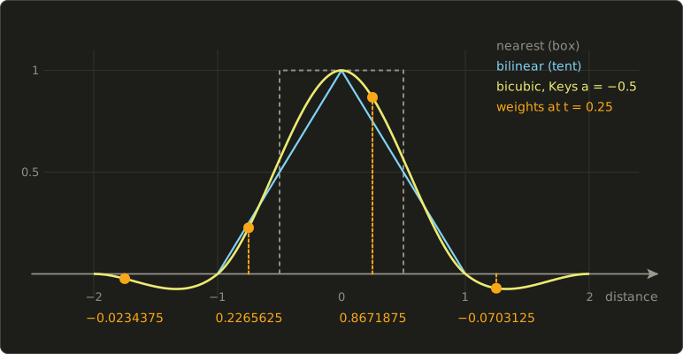
Two cases show what the negative weights do:
- An edge, samples 0, 0, 100, 100: bicubic gives , bilinear gives 25. The bicubic edge is steeper, so it looks sharper.
- Samples 0, 100, 100, 100: bicubic gives , more than any sample. That's an overshoot, the same ringing as in unsharp masking; results must be clamped to the valid range.
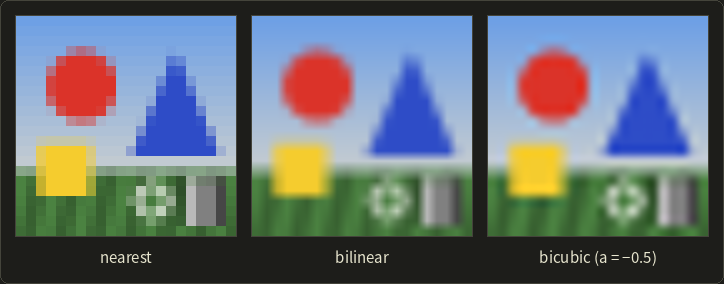
High-quality resizers also use the Lanczos kernel (a windowed sinc, 6 × 6 pixels).
For shrinking, interpolation is not enough: the image must first be low-pass filtered, or fine patterns turn into moiré, the minification problem of mipmaps.
Projective transforms: perspective correction
A photo of a poster or a document taken at an angle shows a rectangle as a general quadrilateral.
The map between the two is a projective transformation (射影変換), or homography (ホモグラフィ), from section 4.4: a 3 × 3 matrix acting on homogeneous coordinates, followed by the division by w:
Multiplying by any nonzero number gives the same mapping, so we may set : 8 unknowns.
Each point pair gives two equations that are linear in the unknowns once the denominator is multiplied out:
So 4 point pairs (no three on one line) give 8 equations, an 8 × 8 linear system, and determine .
That's why "perspective crop" tools ask for four corners.
Worked check with the matrix of section 4.4, which maps the rectangle onto the trapezoid .
Writing down the 8 equations for these four pairs and solving them gives back exactly and all other unknowns 0 (with ): that's .
To rectify the photo (make the poster rectangular again) we use inverse mapping: for each pixel of the straight output, tells us where to read in the photo.
The output point goes to , which after the division is in the photo; there we sample bilinearly.
(Forward mapping would use , which takes the photo's back to the corner .)
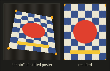
Far-away detail is blurrier after rectification, because fewer photo pixels covered it; homographies between overlapping photos are also the basis of panorama stitching (chapter 16).
Lens distortion correction
Real lenses bend straight lines (section 2.3): barrel distortion pulls the corners in, so straight lines bow outwards (typical of wide-angle lenses), and pincushion distortion pushes them out, so lines bow inwards.
The common model is radial, in coordinates centered on the image and scaled so that is the distance from the center:
where is where the point would be with a perfect pinhole and where the lens actually puts it; is barrel, pincushion.
Worked example. With (and no ), the point at moves to , and the point at moves to : the outer point moves 10% inwards, the inner one only 2.5%.
That uneven scaling is what bends the straight lines.
Inverse mapping makes the correction easy: for each pixel of the corrected image we know , compute with the formula as it is, and read the photo there.
We never need to invert the polynomial, which has no simple closed form.
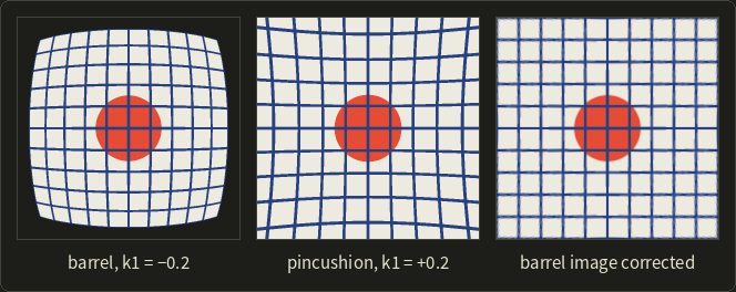
The values come from photographing a checkerboard (camera calibration); VFX undistorts the live-action plate, composites the CG, and distorts the result again (chapter 14).
Warping and morphing
A warp (ワーピング) is a smooth, user-specified mapping of the image plane: by moving the points of a grid laid over the image (mesh warping), or by drawing matching lines in two images (feature-based warping, Beier and Neely, 1992), where each point follows a distance-weighted mix of the lines' transforms.
Morphing (モーフィング) turns image A into image B; a plain cross-dissolve (クロスディゾルブ) only fades: .
Worked example. A pixel that is 200 in A and 40 in B is at .
If the shapes are in different places, a cross-dissolve shows both half transparent ("ghosting"), so a morph first warps both images towards the in-between geometry (each feature moved the fraction of the way from its position in A to its position in B) and then cross-dissolves the warped images:
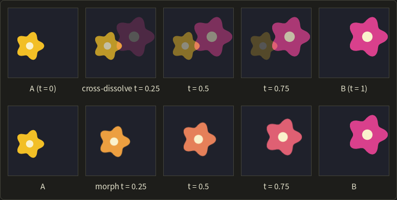
Here the features are just each flower's center and radius, so the warp is a similarity transform; faces need many feature lines.
Morphing is the 2D cousin of the 3D shape interpolation of section 13.5 and of view interpolation (section 12.13).
Exam points
- Forward mapping (input → output) leaves holes when enlarging and overwrites when shrinking; inverse mapping (output → input) gives every output pixel one value and needs interpolation.
- Nearest (1 pixel, blocky), bilinear (2 × 2, smooth but blurry), bicubic (4 × 4, sharper, can overshoot because of negative weights).
- Shrinking needs low-pass filtering first, or it aliases.
- An affine transform has 6 unknowns (3 point pairs); a homography has 8 (4 point pairs, ); perspective correction = homography + inverse mapping.
- Lens distortion: radial model , barrel () and pincushion (); corrected by inverse mapping.
- Morph = warp both images to the in-between geometry + cross-dissolve; a cross-dissolve alone ghosts.
15.7 Image editing
The last syllabus item is what image editors do with all of the above.
Layers and blend modes
A layer combines with the layers below it through a blend mode (描画モード, ブレンドモード).
Write for the value below (the base) and for the layer on top, both from 0 to 1, per channel; the blended result is then mixed into the base with the layer's opacity, using the over operator.
| Mode | Formula | Effect |
|---|---|---|
| normal | b | the top layer covers |
| multiply (乗算) | ab | always darker; white is neutral, black stays black (like stacking slides or filters) |
| screen (スクリーン) | 1 − (1 − a)(1 − b) | always lighter; black is neutral (like two projectors on one screen) |
| overlay (オーバーレイ) | 2ab if a < 0.5, else 1 − 2(1 − a)(1 − b) | more contrast: multiply on dark bases, screen on light ones |
| add (加算) | min(a + b, 1) | light adding up, glows |
| difference (差の絶対値) | the absolute value of a − b | zero where identical; used to compare images |
| darken / lighten (比較(暗)/比較(明)) | min(a, b) / max(a, b) | keep the darker / lighter value per channel |
Worked example. Base , layer :
- multiply: ;
- screen: ;
- overlay: , so the screen branch, ;
- add: ; difference: ; darken: ; lighten: .
With a darker base , overlay uses the multiply branch: .
Multiply and screen are each other's mirror image: screen is multiply applied to the negatives, .
Hard light is overlay with the roles of and swapped (the condition tests the top layer), and soft light is a gentler overlay whose exact formula differs between programs.
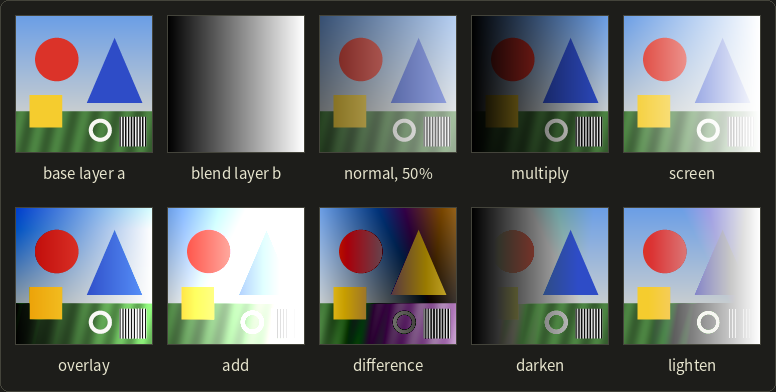
With the ramp, multiply shows the base at the right end (b = 1) and black at the left, screen the reverse.
Most editors apply these to the gamma-encoded values, which is part of their familiar look; compositing software, which models light, works in linear space.
Masks and selections
A mask (マスク) is a gray image that controls where an operation applies: 1 = fully, 0 = not at all, in between = partly.
A selection (選択範囲) is a mask being edited: rectangles, lasso paths, the magic wand (the seed fill of section 6.8 with a color tolerance), color ranges (best in HSV or Lab) and keying (chapter 14).
Selections are feathered (the mask is blurred so the edit fades out) and grown or shrunk with dilation and erosion.
Cloning, healing and Poisson blending
The clone stamp (コピースタンプ) copies pixels from another part of the image at a fixed offset, through a soft brush.
Any difference in brightness or color shows as a patch, so the healing brush (修復ブラシ) copies the texture of the source but takes the brightness and color from the surroundings of the target.
The math behind it is Poisson image editing (ポアソン画像編集, Pérez, Gangnet and Blake, 2003), also called seamless cloning.
Inside the pasted region, instead of the source values, we keep the source's gradients (its edges and texture), and require the result to equal the target on the border of the region.
That's the equation inside the region, with = target on the border: a Poisson equation, solved as a large sparse linear system (one unknown per pixel).
Worked example in 1D.
The target row has the values 100 and 140 on the two border pixels, and we paste three interior pixels from a source row 20, 30, 60, 30, 20 (with its own border values 20 and 20).
Pasting directly gives 100, 30, 60, 30, 140, with two hard jumps.
The source's second differences at the three interior pixels are , and .
We need with the same second differences and , :
The solution is .
Check: , , .
It's the source plus the linear ramp 80, 90, 100, 110, 120: the source's bump survives and meets both borders without jumps (in 2D the correction is the smoothest surface matching the border).
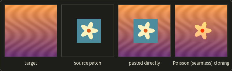
The patch's flat background disappears (it had no gradients); the star keeps its shape but takes on the sunset's colors.
Inpainting
Inpainting (インペインティング) fills a hole with no source at all, from the surroundings only.
The simplest version is the Poisson equation with zero guidance, : the hole is filled with the smoothest surface that matches its border (in the 1D example, 110, 120, 130 between 100 and 140).
That works for scratches and dust but blurs larger holes.
Exemplar-based inpainting copies matching patches from elsewhere in the image, filling from the edge inwards (Criminisi and colleagues, 2004; made interactive by PatchMatch, 2009, as "content-aware fill"), and today generative neural networks invent content for large holes.
Retouching in practice
A typical retouch uses the whole chapter: curves and white balance; cloning, healing and inpainting; dodge and burn (local brightening and darkening painted as a mask); frequency separation (a low-pass and a high-pass layer retouched separately, the Laplacian pyramid in two levels); and sharpening as the last step.
Professionals work non-destructively (adjustment layers and masks that can be changed later) and in 16 bits per channel, so that repeated tone changes don't create false contours.
Exam points
- Multiply darkens (white neutral), screen lightens (black neutral), overlay = multiply below 0.5, screen above (based on the lower layer); hard light tests the upper layer.
- Masks control where an operation applies; feathering = blurring the mask.
- Clone stamp copies pixels; healing and Poisson blending copy gradients and match the surroundings ( with the target on the border).
- Inpainting fills holes from the surroundings: diffusion () for small holes, patch-based for larger ones.
15.8 Summary
- A digital image is an array of values; operations are per-pixel, local, geometric or global. The histogram counts pixels per level; mean and variance measure brightness and contrast.
- Binary images use 4- or 8-neighborhoods; HDR images store linear floating-point light (OpenEXR, Radiance RGBE); pyramids store several resolutions (Gaussian) or frequency bands (Laplacian).
- 2D drawing: rasterization with coverage-based anti-aliasing, Bézier paths filled with the even-odd or nonzero rule, outline fonts, brush stamps, layers composited with (premultiplied) alpha.
- Tone curves (stretch, negative, gamma, posterize) are applied as LUTs; Otsu maximizes the between-class variance; equalization uses the cumulative histogram as the curve.
- Color conversion uses weighted sums and 3 × 3 matrices or HSV; tone mapping compresses HDR to the display (exposure, key 0.18, Reinhard ).
- Filters: box and Gaussian smoothing (separable), median for impulse noise, Prewitt/Sobel gradients, the Laplacian and zero crossings, unsharp masking, the bilateral filter and binary morphology; smoothing is low-pass, edge detection high-pass.
- Geometric transforms use inverse mapping plus resampling (nearest, bilinear, bicubic); homographies from 4 point pairs fix perspective; radial models fix lens distortion; morphing = warping + cross-dissolve.
- Editing: blend modes (multiply, screen, overlay, …), masks and selections, cloning and Poisson-based healing, inpainting.
15.9 Key terms
| English | 日本語 |
|---|---|
| image processing | 画像処理 |
| histogram | ヒストグラム |
| cumulative histogram | 累積ヒストグラム |
| mean / variance / standard deviation | 平均/分散/標準偏差 |
| binary image | 二値画像 |
| 4-neighborhood / 8-neighborhood | 4近傍/8近傍 |
| connected component / labeling | 連結成分/ラベリング |
| dynamic range | ダイナミックレンジ |
| high dynamic range (HDR) image | ハイダイナミックレンジ画像(HDR画像) |
| multi-resolution, image pyramid | 多重解像度、画像ピラミッド |
| Gaussian pyramid / Laplacian pyramid | ガウシアンピラミッド/ラプラシアンピラミッド |
| anti-aliased drawing | アンチエイリアス描画 |
| path | パス |
| even-odd rule / nonzero winding rule | 偶奇規則/非ゼロ回転数規則 |
| winding number | 回転数 |
| outline font / bitmap font | アウトラインフォント/ビットマップフォント |
| hinting | ヒンティング |
| layer | レイヤー |
| premultiplied alpha | 乗算済みアルファ(プリマルチプライドアルファ) |
| tone (gray-level) conversion | 濃淡変換 |
| tone curve | トーンカーブ |
| linear stretch | 線型の引き伸ばし(コントラスト伸張) |
| negative | ネガ(反転) |
| gamma conversion | ガンマ変換 |
| posterization | ポスタリゼーション |
| lookup table (LUT) | ルックアップテーブル(LUT) |
| binarization / threshold | 二値化/しきい値 |
| Otsu's method | 大津の方法(判別分析法) |
| between-class variance | クラス間分散 |
| histogram equalization | ヒストグラム平坦化(均等化) |
| color conversion | 色変換 |
| saturation / hue | 彩度/色相 |
| sepia | セピア |
| tone mapping | トーンマッピング |
| exposure | 露出 |
| key value / log-average luminance | キー値/対数平均輝度 |
| spatial filtering | 空間フィルタリング |
| kernel | カーネル(フィルタ係数) |
| convolution / correlation | 畳み込み/相関 |
| smoothing | 平滑化 |
| mean (box) filter | 平均値フィルタ(ボックスフィルタ) |
| Gaussian filter | ガウシアンフィルタ |
| separable filter | 分離可能なフィルタ |
| median filter | メディアンフィルタ |
| Gaussian noise / salt-and-pepper noise | ガウスノイズ/ごま塩ノイズ |
| edge detection | エッジ検出 |
| gradient | 勾配 |
| differential filter | 微分フィルタ |
| Prewitt filter | プリューウィットフィルタ |
| Sobel filter | ソーベルフィルタ |
| Laplacian filter | ラプラシアンフィルタ |
| zero crossing | ゼロ交差 |
| Laplacian of Gaussian (LoG) | LoGフィルタ |
| Canny edge detector | キャニー法 |
| sharpening | 鮮鋭化 |
| unsharp masking | アンシャープマスキング |
| bilateral filter | バイラテラルフィルタ |
| morphology | モルフォロジー |
| structuring element | 構造要素 |
| dilation / erosion | 膨張/収縮 |
| opening / closing | オープニング/クロージング |
| Fourier transform | フーリエ変換 |
| convolution theorem | 畳み込み定理 |
| low-pass filter / high-pass filter | ローパスフィルタ/ハイパスフィルタ |
| geometric transformation | 幾何学的変換 |
| forward mapping / inverse mapping | 順方向マッピング/逆方向マッピング |
| resampling | 再標本化(リサンプリング) |
| nearest-neighbor interpolation | 最近傍補間(ニアレストネイバー) |
| bilinear interpolation | 双線型補間(バイリニア補間) |
| bicubic interpolation | 双三次補間(バイキュービック補間) |
| projective transformation, homography | 射影変換、ホモグラフィ |
| lens distortion (barrel, pincushion) | 歪曲収差(樽型、糸巻き型) |
| warping | ワーピング |
| morphing / cross-dissolve | モーフィング/クロスディゾルブ |
| blend mode | 描画モード(ブレンドモード) |
| multiply / screen / overlay | 乗算/スクリーン/オーバーレイ |
| mask / selection | マスク/選択範囲 |
| clone stamp / healing brush | コピースタンプ/修復ブラシ |
| Poisson image editing | ポアソン画像編集 |
| inpainting | インペインティング |
15.10 Challenges
- ★ A 4 × 4 image with 4 levels (0 to 3) has the histogram . Compute its mean and variance, the equalization table and the new histogram, and find Otsu's threshold from the between-class variances for .
- ★ A 3 × 3 window holds 20 30 40 / 30 200 50 / 40 50 60. Compute the center's output for the 3 × 3 mean filter, the 1 2 1 Gaussian of section 15.5, the median filter and the 4-neighbor Laplacian, and the Sobel , , gradient magnitude and direction. Which value would you call the "noise-free" estimate, and why?
- ★★ Compute the bicubic weights () at and interpolate between the samples 0, 20, 60, 100 (at positions −1, 0, 1, 2). Compare with bilinear interpolation, and explain why the bicubic result lies below the linear one here.
- ★★ Four HDR pixels have the luminances 0.05, 0.2, 0.8 and 3.2. Compute the log-average luminance (it's a round number), the scaled luminances for the key 0.18 and the Reinhard results . How many stops is the range of the input?
- ★★★ Show that unsharp masking with the blur and is the same as (1D second difference), and check it on the profile of section 15.5. Then find two 3-pixel signals , for which the median of is not the sum of the medians, and explain why that proves the median filter has no kernel.
- ★★ A row of 4 pixels (positions 0 to 3) is enlarged by 1.5 with forward mapping . Which of the output pixels 0 to 5 receive a value? Then do it with inverse mapping and nearest-neighbor rounding, and list which input pixel each output pixel reads.
Multiple choice
Q1 ★ Which of the following statements about spatial filtering is correct?
| A | The Sobel filter is a second-derivative filter whose zero crossings mark the edges. |
| B | The Gaussian filter gives all pixels in its window the same weight. |
| C | Unsharp masking blurs the image in order to reduce noise. |
| D | The Laplacian filter is insensitive to noise because it treats all directions equally. |
| E | The median filter removes salt-and-pepper noise well and keeps edges sharper than the mean filter. |
Q2 ★ Which of the following statements about gray-level conversion is correct?
| A | Histogram equalization always produces a perfectly flat histogram. |
| B | Histogram equalization uses the normalized cumulative histogram as the tone curve, and it never increases the number of distinct gray levels. |
| C | Otsu's method chooses the threshold that minimizes the between-class variance. |
| D | The negative of an image has the same histogram as the original image. |
| E | Binarization with a fixed threshold automatically adapts to the overall brightness of the image. |
Q3 ★★ An image is rotated and enlarged. Which of the following statements is correct?
| A | Forward mapping never leaves holes when an image is enlarged. |
| B | Bicubic interpolation uses the 2 × 2 pixels around the sampling position. |
| C | A projective transformation (homography) is fully determined by 3 pairs of corresponding points. |
| D | Inverse mapping computes, for each output pixel, its position in the input image and interpolates there, so the output has no holes. |
| E | Bilinear interpolation can produce values larger than the largest of the four pixels it uses. |
15.11 Practical assignment
Process one small image by hand through the main steps of this chapter, and check every step with a property it must satisfy.
You need graph paper, a pencil, colored pencils and a calculator.
The image is 6 × 6 pixels with 8 levels (0 to 7), row 0 at the top:
| col 0 | col 1 | col 2 | col 3 | col 4 | col 5 | |
|---|---|---|---|---|---|---|
| row 0 | 6 | 6 | 5 | 6 | 6 | 6 |
| row 1 | 6 | 5 | 6 | 6 | 5 | 6 |
| row 2 | 6 | 6 | 1 | 2 | 1 | 6 |
| row 3 | 5 | 6 | 2 | 7 | 2 | 6 |
| row 4 | 6 | 6 | 1 | 2 | 1 | 6 |
| row 5 | 6 | 0 | 6 | 6 | 6 | 5 |
It's a dark 3 × 3 object on a light background, with one bright noise pixel inside the object and one dark noise pixel in the background.
- Step 1: Draw the image on graph paper (2 × 2 squares per pixel), shading each pixel with your pencil (0 = darkest).
- Step 2: Histogram. Count for , draw it as a bar chart, and compute the cumulative histogram, the mean and the variance.
- Step 3: Otsu. For every threshold compute , , , and in a table. Choose and draw the binary image (dark class = object). Which pixels are classified wrongly?
- Step 4: Median. Apply the 3 × 3 median filter (clamp at the borders) to all 36 pixels and draw the result. Binarize it with the same and compare with step 3.
- Step 5: Sobel. On the original image, compute , and the gradient magnitude at row 2, column 1 (on the object's left edge) and at row 1, column 2 (above it). Draw the gradient vectors as arrows on your drawing.
- Step 6: Equalization. Compute the table and the histogram of the equalized image.
- Step 7: Enlarge. The image is enlarged 2× by inverse mapping, (and the same for y). Compute the bilinear value of the output pixel at , .
How to check yourself:
- Step 2: the histogram adds up to 36 and the cumulative histogram ends at 36; the mean lies between the two humps.
- Step 3: levels 3 and 4 are empty, so several thresholds give the same and the same binary image; for your , the weighted within-class variances plus must equal the variance from step 2. Exactly two pixels are wrong (the two noise pixels).
- Step 4: both noise pixels are gone, but the object is no longer a square; explain what happened to its four corner pixels (look at how many dark pixels their windows contain). This is why opening and closing (section 15.5) exist.
- Step 5: the arrows point from the dark object towards the light background, perpendicular to the object's edge; inside a constant area the magnitude is 0.
- Step 6: the table never decreases, the brightest occupied level goes to 7, and the equalized histogram has no more nonzero bars than the original one.
- Step 7: the result lies between the smallest and the largest of the four pixels you used.
コメント(0)
まだコメントはありません。
ログインするとコメント出来ます。