29. Modern GPU Systems and Neural Rendering
This is the last chapter of Part 2, and it looks at where graphics is going: the machines that run it today and the neural networks that have started to render with it.
Chapter 17 introduced the GPU as a throughput machine with warps, branch divergence and limited bandwidth, and its forward and deferred renderers; chapter 12 ended its tour of image-based rendering with NeRF and 3D Gaussian splatting and promised them here; chapter 20 and chapter 23 pointed here for neural upscalers and denoisers.
This chapter keeps those promises.
The first half is about modern GPU systems: occupancy and latency hiding, explicit APIs, mesh shaders and GPU-driven rendering, hardware ray tracing, and lighting architectures.
The second half is about neural rendering: neural networks in one page, upscaling and frame generation, NeRF, hash grids, 3D Gaussian splatting, neural textures and generative models.
It ends with what to learn next and a look back at Part 2, before the mini-exam of chapter 30.
This is Part 2 material and goes beyond the exam syllabus, but it deepens two of its items: real-time 3D CG systems (リアルタイム3次元CGシステム, chapter 17) and image-based rendering (イメージベーストレンダリング, chapter 12).
Current technology changes fast.
Read every product, API version and number about real hardware as "at the time of writing" (late 2026); product names such as DLSS, FSR, XeSS or Nanite appear only as examples, not as recommendations.
We'll use matrix–vector products (Linear Algebra chapter 6), the transpose (chapter 7) and quaternions (chapter 13), the volume rendering of chapter 28 and the front-to-back compositing of section 20.8.
29.1 Inside a modern GPU
Warps, again
Section 17.2 described the GPU as many small lanes grouped into blocks (streaming multiprocessors or compute units), running in lock-step groups of 32 or 64 called warps (ワープ) or wavefronts (ウェーブフロント), and showed that a divergent branch runs both paths.
Two more things decide a shader's speed: where its data lives, and how many warps are ready at once.
The memory hierarchy
Rough orders of magnitude at the time of writing (they vary by vendor and generation):
| Level | Typical size | Shared by | Rough latency |
|---|---|---|---|
| registers | 64K 32-bit registers per block | one thread (lane) | about 1 cycle |
| shared memory (LDS) | tens of KB to about 100 KB per block | one workgroup | tens of cycles |
| L1 / texture cache | similar, often the same storage as shared memory | one block | tens of cycles |
| L2 cache | a few MB to about 100 MB | the whole GPU | a few hundred cycles |
| VRAM (GDDR, HBM) | 8 to 32 GB on consumer cards | the whole GPU | several hundred cycles |
Registers (レジスタ) are private to each thread, and a block's register file is fixed: more registers per thread means fewer threads.
Shared memory (共有メモリ, LDS on AMD) is a scratchpad shared by the threads of one workgroup, the tool for reductions, tiled filters and the light lists of section 29.5.
Occupancy, worked
The GPU's answer to latency is the one from chapter 17: keep many warps resident on each block and switch to a ready one whenever the current one waits.
Occupancy (占有率, オキュパンシー) is the number of resident warps divided by the maximum the block supports.
Three resources limit it: the register file, the shared memory, and a hardware maximum of warps (and workgroups) per block.
Take an example block similar to recent desktop GPUs: 65,536 32-bit registers, at most 48 resident warps of 32 threads, 4 warp schedulers (12 warp slots each) and 100 KB of shared memory.
A shader that uses registers per thread needs registers per warp, so
- : , capped at 48 warps, occupancy 100%.
- : warps, occupancy .
- : warps, occupancy .
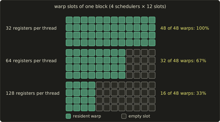
Compute shaders are scheduled in whole workgroups (ワークグループ), so shared memory can be the limit instead.
A workgroup of 256 threads (8 warps) with 40 registers per thread and 24 KB of shared memory fits times by registers but only times by shared memory, so 4 workgroups, 32 warps, 66.7%.
Real GPUs also round register and shared-memory allocations up to fixed granules, which makes the steps coarser; vendor profilers report the exact limiter.
Latency hiding, worked
How many warps are enough?
A simple model: one scheduler issues one instruction per cycle; each warp issues cycles of independent arithmetic, then needs a memory result that takes cycles to arrive.
During one round of cycles a warp keeps the scheduler busy for , so warps keep it busy for a fraction
and full latency hiding (レイテンシ隠蔽) needs warps per scheduler.
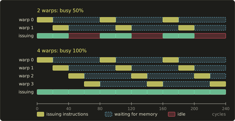
The figure uses and : two warps reach , four reach .
With a more realistic cycles and , full hiding needs warps per scheduler, more than the 12 slots of our block:
- (12 warps per scheduler): ;
- (8 warps per scheduler): ;
- (4 warps per scheduler): .
There are two ways out: more warps (fewer registers), or more independent work per memory access (larger ; with , 8 warps reach ), for example by issuing several texture fetches before using the first result.
Higher occupancy isn't always faster: forcing fewer registers can spill values to slow memory, and bandwidth-bound shaders gain nothing.
Compute shaders and async compute
A compute shader (コンピュートシェーダー) runs a grid of workgroups with no fixed-function stages; its threads read and write buffers directly and cooperate through shared memory inside the workgroup.
In a modern engine much of the frame is compute: culling, light lists, simulation (chapter 26), post-processing, TAA, denoisers and neural networks.
Async compute (非同期コンピュート) submits compute work on a second queue so it can overlap with graphics work that leaves the lanes idle, such as shadow-map rendering; the saving is at most the shorter job, and the two compete for caches and bandwidth.
29.2 Explicit graphics APIs
OpenGL and Direct3D 11 hid a lot of work in the driver (resource tracking, synchronization, compiling shader variants on the fly), mostly on one CPU thread.
The explicit APIs (明示的なAPI) Vulkan (2016), Direct3D 12 (2015) and Metal (2014) hand these decisions to the application:
- Command buffers (コマンドバッファ): draws and dispatches are recorded on as many CPU threads as you like and submitted to a queue later.
- Pipeline state objects (パイプラインステートオブジェクト, PSO): shaders and fixed-function state are compiled together in advance, so nothing compiles mid-frame (when it does anyway, the result is the familiar shader-compilation stutter).
- Barriers (バリア): the application declares, for example, that a render target will next be read by a fragment shader; the GPU waits, flushes caches and may change the image layout. Too few corrupt images, too many serialize the GPU.
- Descriptors (デスクリプタ): small records that tell a shader where a buffer or texture is. Instead of binding a few textures per draw, bindless (バインドレス) rendering puts thousands of descriptors into one big array and lets each draw pass only an index, which is what makes the GPU-driven rendering of section 29.3 possible.
Worked example (illustrative numbers). A scene has 10,000 draws per frame, and recording one costs the application 2 µs of CPU time.
On one thread that's µs = 20 ms, more than a whole 60 fps frame; on 8 threads it's ms.
The price is responsibility: memory allocation, CPU–GPU synchronization (fences and semaphores) and every barrier are now the application's job, which is why the OpenGL series of this site starts with the friendlier model.
29.3 Mesh shaders and GPU-driven rendering
Mesh shaders and meshlets
The classic geometry pipeline of chapter 6 reads an index buffer with a fixed-function input assembler and runs the vertex shader once per vertex.
Mesh shaders (メッシュシェーダー) replace that front end with two compute-like stages:
- a task shader (タスクシェーダー; amplification shader in Direct3D) runs per group of clusters, can cull whole clusters or pick a level of detail, and decides how many mesh shader workgroups to launch;
- a mesh shader workgroup outputs a small mesh directly, its vertices and its triangles, to the rasterizer.
The unit of work is a meshlet (メッシュレット): a cluster of neighboring triangles with a small vertex list.
NVIDIA's introduction of Turing mesh shaders (September 2018) recommended up to 64 vertices and 126 triangles per meshlet; Direct3D 12 added mesh shaders with DirectX 12 Ultimate (March 2020), Vulkan with the cross-vendor VK_EXT_mesh_shader (September 2022), and Metal 3 (2022) has them too.
Worked example. An 8 × 8 grid of vertices is one meshlet of 64 vertices and triangles.
A classic 32-bit index buffer stores bytes for it.
A meshlet stores 64 global vertex indices ( bytes), then three 8-bit local indices per triangle ( bytes) and a 16-byte descriptor: bytes, 48% of the original.
Real meshes save less (NVIDIA's article reports typically about 75% of the original index buffer); the bigger win is that each meshlet carries a bounding sphere and a normal cone and can be culled as a whole.
GPU-driven culling
In a GPU-driven renderer (GPU駆動レンダリング), the list of objects lives on the GPU, and compute shaders decide what to draw:
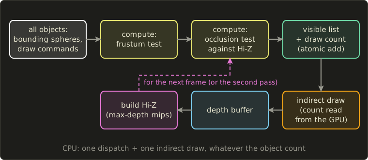
- A compute shader tests every object's bounding sphere against the six planes of the view frustum (section 6.4).
- Survivors are tested against a Hi-Z pyramid (階層Z): a mip chain of the depth buffer whose texels keep the farthest depth below them, like the tiles of hierarchical Z in section 19.5: if the object's nearest depth is behind the farthest depth stored in the texels it covers, it's hidden.
- Each visible object appends its draw command to a buffer with an atomic counter.
- An indirect draw (インダイレクト描画) such as Vulkan's
vkCmdDrawIndexedIndirectCountreads the commands and their count from GPU memory, so the CPU never sees the result.
Hi-Z needs a depth buffer before the frame is drawn.
The common two-phase scheme draws last frame's visible objects first, builds Hi-Z from that depth, tests everything else against it, and draws the newly visible objects in a second pass.
Worked example: the sphere–plane test. In view space the camera looks down with a 90° horizontal field of view.
The left plane passes through the origin, and its unit normal pointing into the frustum is (the point gives , inside).
A sphere with center and radius is completely outside when (here ):
- , : , culled.
- , : , kept (it straddles the plane).
For the occlusion test, a sphere that projects to a 40 × 40-pixel rectangle is checked at Hi-Z mip level , where a texel covers 64 × 64 pixels, so at most 2 × 2 texels have to be read.
Here is the frustum part as a compute shader:
struct DrawCommand {
  uint indexCount; uint instanceCount; uint firstIndex; int vertexOffset; uint firstInstance;
};
struct Frustum { float4 planes[6]; uint objectCount; };

StructuredBuffer<float4> spheres;            // xyz = center in view space, w = radius
StructuredBuffer<DrawCommand> allDraws;
RWStructuredBuffer<DrawCommand> visibleDraws;
RWStructuredBuffer<uint> drawCount;          // reset to 0 before the dispatch
ConstantBuffer<Frustum> frustum;

[shader("compute")]
[numthreads(64, 1, 1)]
void cullMain(uint3 id : SV_DispatchThreadID) {
  uint i = id.x;
  if (i >= frustum.objectCount) return;
  float4 s = spheres[i];
  for (int k = 0; k < 6; ++k) {
    if (dot(frustum.planes[k].xyz, s.xyz) + frustum.planes[k].w < -s.w) return;
  }
  uint slot;
  InterlockedAdd(drawCount[0], 1u, slot);
  visibleDraws[slot] = allDraws[i];
}
#version 450
layout(local_size_x = 64) in;
struct DrawCommand {
uint indexCount; uint instanceCount; uint firstIndex; int vertexOffset; uint firstInstance;
};
layout(std430, set = 0, binding = 0) readonly buffer Spheres { vec4 spheres[]; }; // center, radius
layout(std430, set = 0, binding = 1) readonly buffer AllDraws { DrawCommand allDraws[]; };
layout(std430, set = 0, binding = 2) writeonly buffer VisibleDraws { DrawCommand visibleDraws[]; };
layout(std430, set = 0, binding = 3) buffer DrawCount { uint drawCount; }; // reset to 0 before
layout(set = 0, binding = 4) uniform Frustum { vec4 planes[6]; uint objectCount; };
void main() {
uint i = gl_GlobalInvocationID.x;
if (i >= objectCount) return;
vec4 s = spheres[i];
for (int k = 0; k < 6; ++k) {
if (dot(planes[k].xyz, s.xyz) + planes[k].w < -s.w) return;
}
uint slot = atomicAdd(drawCount, 1u);
visibleDraws[slot] = allDraws[i];
}struct DrawCommand {
uint indexCount; uint instanceCount; uint firstIndex; int vertexOffset; uint firstInstance;
};
struct Frustum { float4 planes[6]; uint objectCount; };
StructuredBuffer<float4> spheres; // xyz = center in view space, w = radius
StructuredBuffer<DrawCommand> allDraws;
RWStructuredBuffer<DrawCommand> visibleDraws;
RWStructuredBuffer<uint> drawCount; // reset to 0 before the dispatch
ConstantBuffer<Frustum> frustum;
[numthreads(64, 1, 1)]
void cullMain(uint3 id : SV_DispatchThreadID) {
uint i = id.x;
if (i >= frustum.objectCount) return;
float4 s = spheres[i];
for (int k = 0; k < 6; ++k) {
if (dot(frustum.planes[k].xyz, s.xyz) + frustum.planes[k].w < -s.w) return;
}
uint slot;
InterlockedAdd(drawCount[0], 1u, slot);
visibleDraws[slot] = allDraws[i];
}The order of the visible draws changes from frame to frame because of the atomic counter; that's fine for opaque geometry with a depth buffer, but transparent objects still need sorting (chapter 20).
Virtualized geometry
Take the idea to its end and the whole mesh becomes a hierarchy of clusters: virtualized geometry (仮想化ジオメトリ).
The best-known example at the time of writing is Nanite in Unreal Engine 5, described by Brian Karis at SIGGRAPH 2021: meshes are split into clusters of about 128 triangles, groups of neighboring clusters are simplified together (with the boundary locked, so cracks can't appear) to about half as many triangles and split into new clusters, and so on up to a root.
At run time a compute pass selects the coarsest clusters whose error projects to less than about one pixel, and only those are streamed in and drawn.
A one-pixel triangle wastes three of the four lanes of its 2 × 2 quad (section 19.5), so the tiny ones are rasterized in a compute shader, writing depth and triangle ID packed in 64 bits with atomic max into a visibility buffer (ビジビリティバッファ; Burns and Hunt, 2013) that a later pass shades.
Worked example: picking the level. Chapter 18 (section 18.5) showed that with a 60° vertical field of view on a 1080-line screen, a length at distance covers about pixels.
A statue of one million triangles has a finest level with an error of 1 cm, and every coarser level halves the triangles and doubles the error.
Level has an error of m, which stays below one pixel while m: level 0 from 9.35 m, level 1 from 18.7 m, level 2 from 37.4 m, level 3 from 74.8 m.
At 75 m the renderer can use level 3, triangles, with no visible difference; the number of triangles drawn follows the number of pixels the object covers, not the size of the source mesh.
Virtual texturing
Textures get the same treatment: virtual texturing (仮想テクスチャ) splits a huge texture into pages, keeps only the pages that recent frames needed in a physical cache texture, and translates addresses through a page table.
A feedback pass (or, with hardware support, sampler feedback) records which pages and mip levels were requested, and missing pages are streamed in, falling back to a coarser mip until they arrive.
Worked example. A virtual texture of RGBA8 texels is 64 GiB; with 128 × 128-texel pages (64 KiB each) it has pages.
A 1920 × 1080 frame needs roughly one texel per pixel, pages' worth; with borders and mip levels a few hundred are typical, and a 4096 × 4096 cache (64 MiB) holds 1024.
29.4 Hardware ray tracing
Two levels of acceleration structures
Section 12.9 built a BVH over triangles and noted that the ray tracing APIs use two levels.
Microsoft announced DirectX Raytracing (DXR) in March 2018, the same year the first GPUs with ray tracing units shipped, and Khronos finalized the Vulkan ray tracing extensions in November 2020.
Both use the same structure:
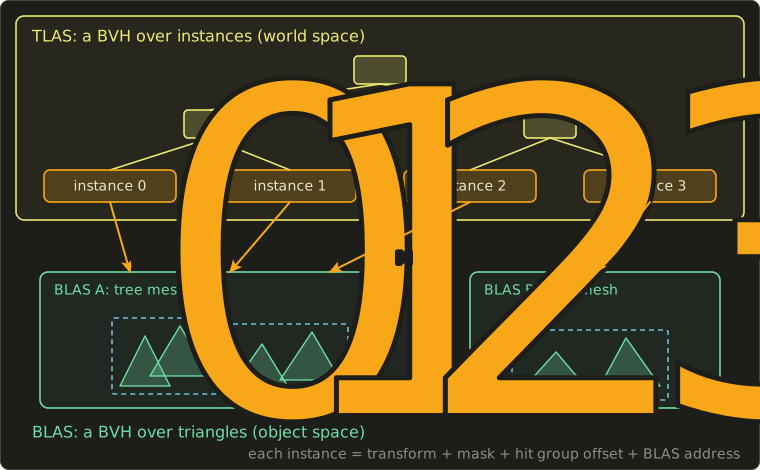
- A BLAS (bottom-level acceleration structure, ボトムレベル加速構造) is a BVH over the triangles (or procedural boxes) of one mesh, in object space.
- A TLAS (top-level acceleration structure, トップレベル加速構造) is a BVH over instances; each instance stores a 3 × 4 transform, a mask, an ID, an offset into the shader table and the address of its BLAS.
A ray first traverses the TLAS in world space; when it reaches an instance, it's transformed into that instance's object space with the inverse transform and continues in the BLAS.
Instancing is therefore nearly free.
Worked example. A forest of 10,000 trees uses one BLAS of 50,000 triangles.
An instance record is 64 bytes in both Direct3D 12 and Vulkan (48 bytes of transform, 8 bytes of ID, mask, offset and flags, and an 8-byte address), so the instances need bytes, 625 KiB, for triangles in the scene.
Moving objects only change their transforms in the small TLAS, rebuilt every frame; deforming meshes refit their BLAS (adjust the boxes, keep the tree), which degrades as the shape drifts, so engines rebuild now and then.
The ray tracing pipeline
The ray tracing pipeline has its own shader stages:
- ray generation (レイ生成シェーダー): one invocation per pixel or per task; it calls
TraceRay()(traceRayEXTin GLSL); - intersection (交差シェーダー): only for procedural geometry such as spheres or SDFs (chapter 21);
- any-hit (任意ヒットシェーダー): runs for candidate hits, typically for alpha testing of leaves and fences;
- closest-hit (最近接ヒットシェーダー): runs once for the nearest hit and does the shading, possibly tracing more rays;
- miss (ミスシェーダー): runs when nothing is hit, for example to sample the sky.
Different objects need different hit shaders, so the shaders are listed in a shader binding table (シェーダーバインディングテーブル, SBT), and the GPU computes which record to run from numbers supplied by the ray and the instance.
In both DXR and Vulkan the hit-group record index is
Worked example. A renderer traces two kinds of rays, primary (offset 0) and shadow (offset 1), so the stride is 2 records per geometry.
A shadow ray hits geometry 1 of an instance whose instance offset is 6: the GPU runs record .
Ray queries
Since DXR 1.1 (2020) and in Vulkan's VK_KHR_ray_query, any shader stage can also trace a ray inline with a ray query (レイクエリ) and look at the result itself, without the separate pipeline and its shader table.
That fits simple questions with one answer, such as a shadow test in a fragment or compute shader:
RaytracingAccelerationStructure sceneTlas;

// Returns true when something blocks the segment from p towards the light.
bool inShadow(float3 p, float3 dirToLight, float maxDist) {
  RayDesc ray;
  ray.Origin = p;
  ray.TMin = 0.001;
  ray.Direction = dirToLight;
  ray.TMax = maxDist;
  RayQuery<RAY_FLAG_ACCEPT_FIRST_HIT_AND_END_SEARCH | RAY_FLAG_FORCE_OPAQUE> q;
  q.TraceRayInline(sceneTlas, RAY_FLAG_NONE, 0xFF, ray);
  while (q.Proceed()) {}
  return q.CommittedStatus() == COMMITTED_TRIANGLE_HIT;
}
#extension GL_EXT_ray_query : require
layout(set = 0, binding = 0) uniform accelerationStructureEXT sceneTlas;
// Returns true when something blocks the segment from p towards the light.
bool inShadow(vec3 p, vec3 dirToLight, float maxDist) {
rayQueryEXT q;
rayQueryInitializeEXT(q, sceneTlas, gl_RayFlagsTerminateOnFirstHitEXT | gl_RayFlagsOpaqueEXT,
0xFF, p, 0.001, dirToLight, maxDist);
while (rayQueryProceedEXT(q)) {}
return rayQueryGetIntersectionTypeEXT(q, true) != gl_RayQueryCommittedIntersectionNoneEXT;
}RaytracingAccelerationStructure sceneTlas;
// Returns true when something blocks the segment from p towards the light.
bool inShadow(float3 p, float3 dirToLight, float maxDist) {
RayDesc ray;
ray.Origin = p;
ray.TMin = 0.001;
ray.Direction = dirToLight;
ray.TMax = maxDist;
RayQuery<RAY_FLAG_ACCEPT_FIRST_HIT_AND_END_SEARCH | RAY_FLAG_FORCE_OPAQUE> q;
q.TraceRayInline(sceneTlas, RAY_FLAG_NONE, 0xFF, ray);
while (q.Proceed()) {}
return q.CommittedStatus() == COMMITTED_TRIANGLE_HIT;
}
Both forms suffer from divergence: neighboring rays of a glossy reflection or a GI bounce hit different materials, and a warp then runs several closest-hit shaders one after the other (section 17.2).
Shader execution reordering (SER) lets the GPU regroup rays by the shader they're about to run, and opacity micromaps (OMM) store per-micro-triangle opacity so alpha-tested foliage needs fewer any-hit invocations; both became part of DXR 1.2, announced in March 2025.
Worked example: the ray budget. At 2560 × 1440 (3,686,400 pixels) and 60 fps, one reflection ray, one shadow ray and one GI ray per pixel are rays per second, about 0.66 billion.
That's why games trace about one sample per pixel and rely on the denoisers and reservoir resampling of chapters 23 and 24.
29.5 Shading rates and lighting architectures
Variable rate shading
Not every pixel needs its own fragment shader invocation: a motion-blurred area, the sky behind fog, or the periphery of a VR lens (section 18.5) look the same when shaded more coarsely.
Variable rate shading (可変レートシェーディング, VRS), available on GPUs since 2018 and exposed in Direct3D 12 and Vulkan, shades once per 1 × 2, 2 × 1, 2 × 2 (and on some hardware 2 × 4, 4 × 2, 4 × 4) block of pixels while keeping full-resolution coverage and depth, so edges stay sharp.
The rate can be set per draw, per triangle, or with a small shading rate image whose texels each cover a tile of 8 × 8 or 16 × 16 pixels.
Worked example. At 2560 × 1440, 40% of the screen is shaded at 2 × 2, 20% at 2 × 1 and 40% at full rate.
The relative number of invocations is , a saving of 40% of the shading work.
A rate image with 16 × 16 tiles has texels.
Forward+, clustered shading and the visibility buffer
Section 17.4 compared forward and deferred rendering and mentioned tiled and clustered shading.
Tiled forward shading or Forward+ (タイルドフォワード; Harada, McKee and Yang, 2012) first renders depth only, then a compute pass divides the screen into tiles (for example 16 × 16 pixels), finds each tile's minimum and maximum depth, and builds a list of the lights whose spheres intersect the tile's small frustum; the forward pass then loops over its tile's list only.
Clustered shading (クラスタードシェーディング; Olsson, Billeter and Assarsson, 2012) divides the view frustum in depth as well, into 3D cells called clusters, independent of the depth buffer, so it also works for transparent surfaces and volumetric fog.
Depth slices are usually spaced exponentially, so that clusters stay roughly cube-shaped:
Worked example. A 1920 × 1080 screen with 64 × 64-pixel tiles has tiles; with slices from to m that's clusters.
Each slice is times deeper than the previous one.
A light of radius 5 m at depth 20 m spans 15 to 25 m, that is to : slices 13 and 14 only, so with 200 lights a pixel loops over a handful instead of 200.
The visibility buffer of section 29.3 is a third way: it stores only a triangle ID per pixel and shades each pixel once by fetching the triangle again, writing far fewer bytes than a G-buffer.
| Architecture | Lighting cost depends on | Transparency | MSAA | Memory per pixel |
|---|---|---|---|---|
| forward | lights × overdraw | natural | natural | small |
| deferred | lights × pixels | separate forward pass | expensive | large G-buffer |
| tiled / clustered forward | lights per tile or cluster × pixels | clustered: natural | natural | small, plus light lists |
| visibility buffer | lights per cluster × pixels | separate pass | possible | very small |
Exam points
These tie back to syllabus area 8, real-time 3D CG systems (chapter 17):
- Occupancy is limited by registers, shared memory and a maximum number of warps per block; the GPU hides memory latency by switching between resident warps.
- Explicit APIs (Vulkan, Direct3D 12, Metal) record command buffers on many threads and make the application responsible for barriers and synchronization.
- In GPU-driven rendering, compute shaders cull objects and write indirect draw commands; mesh shaders process meshlets instead of single vertices.
- Ray tracing APIs use a TLAS of instances over BLASes of triangles; deferred shading stores a G-buffer, clustered shading bins lights into 3D cells.
29.6 Neural networks in one page
Neurons, layers and the MLP
A neural network (ニューラルネットワーク) is a function with many adjustable numbers, called parameters or weights, which are tuned on examples until the function does what we want.
Its building block, a neuron, computes a weighted sum of its inputs plus a bias and passes it through a nonlinear activation function (活性化関数), most often the ReLU, :
A layer of neurons is a matrix–vector product plus a bias vector, followed by the activation applied to each component, : exactly the matrix–vector multiplication of Linear Algebra chapter 6.
Stacking layers gives a multilayer perceptron (多層パーセプトロン, MLP), the network NeRF uses:
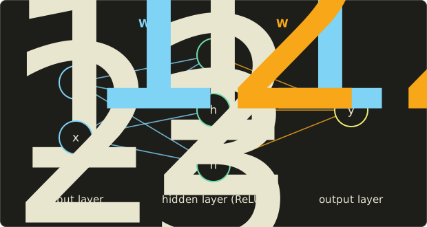
Without the nonlinearity, two layers would collapse into one matrix, ; with it, an MLP that is wide enough can approximate any continuous function on a bounded domain.
Training: loss, gradient, backpropagation
Training (学習) adjusts the parameters to make a loss function (損失関数) small, for example the squared error between the output and the desired value , averaged over many examples.
Gradient descent (勾配降下法) moves every parameter a small step against its derivative, , with a learning rate .
Backpropagation (誤差逆伝播法) computes all these derivatives in one backward pass with the chain rule, layer by layer from the output to the input.
Real training uses random mini-batches and update rules such as Adam; using the trained network is inference (推論).
Worked example: one neuron, one step.
Inputs , weights , bias , target , learning rate .
- Forward: , and . Loss .
- Backward: ; the ReLU passes it unchanged because ; so and .
- Update: , .
- Check: , loss , 25 times smaller.
Why GPUs love it
A layer applied to many inputs is a matrix–matrix product, and a 64 × 64 layer applied to every pixel of a 1920 × 1080 frame costs floating-point operations, about 1.02 TFLOP/s at 60 fps, for one small layer.
That's why recent GPUs have matrix units (chapter 17) that multiply small low-precision matrix tiles many times faster than the ordinary lanes, and why APIs are opening them to ordinary shaders: at the time of writing, Vulkan has cooperative-matrix extensions, and Direct3D's matrix operations for shaders (first previewed as "cooperative vectors") are in preview for Shader Model 6.10.
29.7 Upscaling, frame generation and denoising
Temporal upscaling with a network
Section 20.6 built TAA: jitter the camera by a sub-pixel offset every frame, reproject last frame's output with motion vectors, reject or clamp history that no longer matches, and blend.
Rendering at a lower resolution and accumulating into a larger history is temporal upscaling (時間方向アップスケーリング), also called super resolution (超解像).
The hard part is what TAA decided with hand-written rules: how much history to trust per pixel near edges, thin features and disocclusions.
Neural upscalers learn those decisions from pairs of low-resolution sequences and high-quality references, with TAA's inputs: jittered color, depth, motion vectors, jitter offset and exposure.
At the time of writing, examples are NVIDIA DLSS (a neural network since the first version in 2019, temporal since DLSS 2 in 2020, transformer-based since DLSS 4), AMD FSR (hand-written up to FSR 3, neural since FSR 4 in 2025) and Intel XeSS; chapter 27 discusses single-image super-resolution, which has no history to work with.
Upscalers offer quality modes defined by the ratio of output to render resolution per axis.
Worked example for 3840 × 2160 output, with the per-axis ratios that AMD's documentation gives at the time of writing (other upscalers use similar ones):
| Mode | Ratio per axis | Render resolution | Rendered pixels |
|---|---|---|---|
| Quality | 1.5 | 2560 × 1440 | 44.4% |
| Balanced | 1.7 | 2259 × 1271 | 34.6% |
| Performance | 2.0 | 1920 × 1080 | 25.0% |
| Ultra Performance | 3.0 | 1280 × 720 | 11.1% |
The pixel fraction is : Balanced renders pixels, of 8,294,400.
Each output pixel still needs several samples over time, so the jitter sequence grows with the ratio: AMD's SDK uses phases, 18 for Quality and 32 for Performance, which gives every output pixel about 8 samples per cycle.
If a native 4K frame takes 20 ms, of which 18 ms scale with the pixel count, and the upscaler itself costs 1.5 ms, Performance mode takes about ms.
Frame generation
Frame generation (フレーム生成) goes one step further: it synthesizes whole frames between rendered ones from motion vectors, optical flow (chapter 27) and a network.
Interpolation needs the next rendered frame before it can show the frame in between, so the newest rendered frame has to wait:
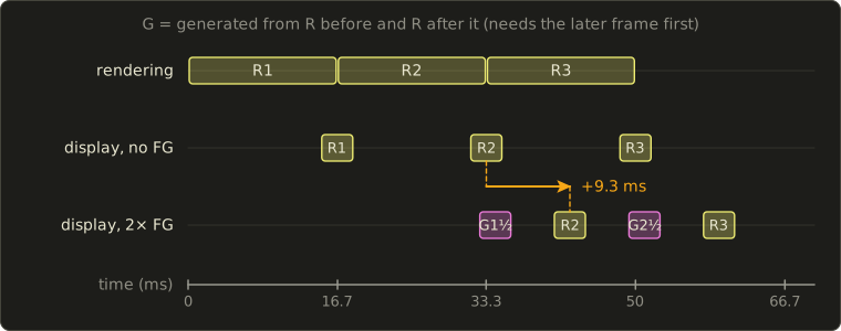
Worked example. The game renders at 60 fps, a frame every 16.7 ms, and generation takes 1 ms.
Without frame generation, R2 is shown when it's done, at 33.3 ms.
With 2× generation, the in-between frame G1½ can only be made once R2 exists, so it appears at ms, and R2 half a display interval later, at ms: 9.3 ms of added latency, while the display shows 120 frames per second.
Multi-frame modes insert several frames: 4× turns 60 rendered frames into 240 displayed ones, one every ms.
The game still reads input 60 times per second, so frame generation improves smoothness, not responsiveness, and its artifacts grow at low base frame rates; vendors pair it with latency-reduction techniques.
At the time of writing NVIDIA's DLSS 4.5 (announced January 2026) offers up to 6× (five generated frames per rendered one), and AMD and Intel offer their own frame generation, also increasingly neural.
Neural denoising
Section 23.12 covered G-buffer-guided denoisers up to neural ones.
The trend in games is one network that denoises the raw ray-traced samples and upscales at once, such as NVIDIA's DLSS Ray Reconstruction (2023) and AMD's FSR Ray Regeneration (2025), and AMD has announced a network that learns the indirect light itself (FSR Radiance Caching).
All of these work in image space; the next sections use networks to represent the scene itself.
29.8 Neural radiance fields (NeRF)
A scene as a function
Section 12.13 described the plenoptic function and light fields: the radiance along every ray, recorded from photos.
NeRF (neural radiance fields, ニューラル放射輝度場; Mildenhall, Srinivasan, Tancik, Barron, Ramamoorthi and Ng, ECCV 2020) stores a scene as a function learned from a few dozen to a few hundred photos with known camera poses:
For a point and a viewing direction it returns a volume density (how much light is absorbed per unit length, which depends only on ) and an emitted color (which may depend on , so highlights move with the view).
are the weights of an MLP.
In the paper, 8 ReLU layers of 256 neurons turn the position into and a feature vector, and one more layer of 128 neurons adds the direction and outputs the color.
Volume rendering along a ray
A pixel's color comes from the emission–absorption model of chapter 28, integrated along the camera ray between a near and a far bound.
NeRF evaluates it at samples with spacings :
is the opacity of the segment around sample , the transmittance (透過率) of everything in front of it, and its weight.
This is exactly the front-to-back under compositing of section 20.8, with each sample as a semi-transparent layer whose alpha comes from a density.
Worked example: compositing one ray.
Five samples at with .
The network returns densities whose are , , , and (that is, ), chosen so the alphas come out round, and the colors are empty, light gray , red , dark red and almost black ; the background is white.
| 1 | 1.0 | 0 | 1 | 0 |
| 2 | 1.5 | 1 | 0.2 | |
| 3 | 2.0 | 0.4 | ||
| 4 | 2.5 | 0.3 | ||
| 5 | 3.0 | 0.5 | 0.05 |
What's left for the background is , and the weights plus that remainder add up to .
The color:
The same weights give an expected depth, , a depth map for free.
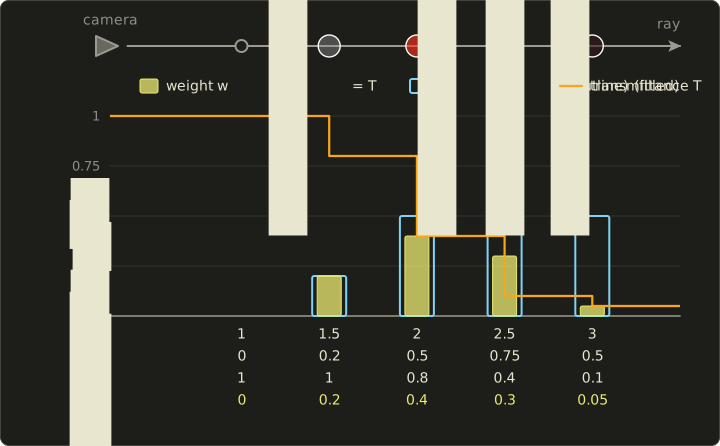
The fifth sample is as opaque as the third but gets an eighth of its weight: 90% of the light was absorbed in front of it.
In code, with the Vec3 of the Linear Algebra series:
#include <cmath>
#include <cstdio>
#include "linalg.hh"

// Composite n samples along one ray, front to back (section 29.8).
// sigmaDelta[i] = sigma_i * delta_i, color[i] = c_i. Returns the pixel color;
// the transmittance that is left at the end is written to *rest.
Vec3 compositeRay(const float *sigmaDelta, const Vec3 *color, int n, Vec3 background,
                  float *rest) {
  Vec3 c = {0.0f, 0.0f, 0.0f};
  float t = 1.0f;                                   // T_i: nothing in front yet
  for (int i = 0; i < n; ++i) {
    float alpha = 1.0f - std::exp(-sigmaDelta[i]);  // alpha_i
    float w = t * alpha;                            // w_i = T_i alpha_i
    std::printf("i=%d alpha=%.3f T=%.3f w=%.3f\n", i, alpha, t, w);
    c = c + w * color[i];
    t = t * (1.0f - alpha);
  }
  *rest = t;
  return c + t * background;
}

int main() {
  // sigma_i delta_i chosen so that alpha = 0, 0.2, 0.5, 0.75, 0.5
  const float sd[5] = {0.0f, std::log(1.25f), std::log(2.0f), std::log(4.0f), std::log(2.0f)};
  const Vec3 col[5] = {{0.0f, 0.0f, 0.0f}, {0.6f, 0.6f, 0.6f}, {1.0f, 0.2f, 0.1f},
                       {0.8f, 0.1f, 0.1f}, {0.2f, 0.1f, 0.1f}};
  float rest;
  Vec3 c = compositeRay(sd, col, 5, {1.0f, 1.0f, 1.0f}, &rest);
  std::printf("color = (%.3f, %.3f, %.3f), T left = %.3f\n", c.x, c.y, c.z, rest);
}
i=0 alpha=0.000 T=1.000 w=0.000
i=1 alpha=0.200 T=1.000 w=0.200
i=2 alpha=0.500 T=0.800 w=0.400
i=3 alpha=0.750 T=0.400 w=0.300
i=4 alpha=0.500 T=0.100 w=0.050
color = (0.820, 0.285, 0.245), T left = 0.050
Training by rendering
Everything in the formula is differentiable, so NeRF trains by rendering: render a random batch of pixels from the photos (4096 rays per step in the paper), compare with a squared error, and backpropagate through the compositing into the MLP.
No geometry is given; density appears where it explains the photos from all directions.
The paper needed 100,000 to 300,000 steps, one to two days per scene on one GPU.
Hierarchical sampling (階層的サンプリング) puts the samples where they matter: a coarse network is evaluated at 64 stratified samples per ray, the weights (normalized to sum to 1) are used as a piecewise-constant probability density, and 128 more samples are drawn from it for a fine network (the importance sampling of chapter 23).
For our ray, the four nonzero weights normalized by 0.95 would attract about , , and of the 128 fine samples: most near the surface at .
Positional encoding
Feed directly into an MLP and the result is blurry.
Networks trained by gradient descent learn low frequencies first and high frequencies very slowly, a spectral bias (スペクトルバイアス; Rahaman and colleagues, 2019).
NeRF's fix is a positional encoding (位置エンコーディング): each coordinate is replaced by sines and cosines of increasing frequency,
with for the position (60 numbers for ) and for the direction (24 numbers).
Tancik and colleagues explained why it works in "Fourier Features Let Networks Learn High Frequency Functions in Low Dimensional Domains" (NeurIPS 2020): the encoded inputs let the network build sharp detail as combinations of fast-varying features instead of having to create them through many layers.
Worked example. With , encodes to , and to .
The input moved by 0.01; the first pair barely changed, but the last pair moved by about 0.25: the high-frequency features make nearby points easy to tell apart.
The effect is easy to reproduce.
The figure shows two small MLPs (two hidden layers of 64 ReLU neurons, trained for 3000 Adam steps on 256 samples of a signal with 2, 9 and 23 cycles) in plain NumPy; one gets , the other with :
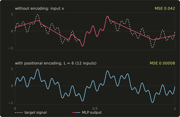
The two networks have almost the same size (4353 and 5057 parameters), but the encoded one reaches an error about 500 times smaller.
Too many frequencies cause the opposite problem: the network invents wiggles between the training samples.
What NeRF costs
The MLP has about 0.6 million weights ( with the layer sizes above and the input re-fed into the fifth layer, as in the paper), and the coarse and fine networks are evaluated times per ray.
An 800 × 800 image is therefore network evaluations, about floating-point operations: more than ten seconds per image even on a GPU that sustains 15 TFLOP/s.
Hundreds of follow-up papers improved quality (anti-aliasing with mip-NeRF, 2021; unbounded and dynamic scenes; relighting) and, above all, speed.
29.9 Instant-NGP and hash grids
The big MLP is doing two jobs: storing where things are and turning that into color and density.
Instant-NGP (Müller, Evans, Schied and Keller, "Instant Neural Graphics Primitives with a Multiresolution Hash Encoding", ACM Transactions on Graphics, SIGGRAPH 2022) moves the storage into trainable tables and keeps only tiny MLPs (64 neurons wide) for the rest.
The multiresolution hash encoding (多重解像度ハッシュエンコーディング) uses grids over the scene, from a coarse resolution to a fine , growing by a constant factor :
Each grid vertex owns a feature vector of trainable numbers.
To encode a point, each level finds the 8 vertices of the cell containing it, looks up their features and interpolates them trilinearly; the 16 levels give numbers, which go into the small MLP.
Fine levels have far more vertices than memory allows, so their vertices are hashed into a table of entries (between and in the paper):
Worked example. With , and : , and the resolutions are 16, 22, 30, 42, 58, 80, 111, 153, 212, 294, 406, 561, 776, 1072, 1482, 2048.
With , a level fits without hashing while : fits, doesn't, so levels 0 to 4 are dense and levels 5 to 15 are hashed.
The tables hold at most parameters, 32 MiB at 2 bytes each (the paper stores them in half precision).
For the vertex of some hashed level, with 32-bit arithmetic that wraps around: and modulo ; ; keeping the low 19 bits gives entry 329,061.
The neighbor lands at 329,058: because , neighbors along differ only in the lowest bits and usually share a cache line.
#include <cstdint>
#include <cstdio>

// Spatial hash of Instant-NGP (section 29.9): XOR of the integer grid
// coordinates times large primes, modulo the table size T (a power of two).
// The products wrap around modulo 2^32, exactly like unsigned 32-bit math on a GPU.
uint32_t gridHash(uint32_t x, uint32_t y, uint32_t z, uint32_t tableSize) {
  const uint32_t p1 = 1u, p2 = 2654435761u, p3 = 805459861u;
  uint32_t h = (x * p1) ^ (y * p2) ^ (z * p3);
  return h & (tableSize - 1u);  // same as h % T when T is a power of two
}

int main() {
  const uint32_t T = 1u << 19;
  std::printf("y * p2 = %u, z * p3 = %u\n", 5u * 2654435761u, 7u * 805459861u);
  std::printf("h(3, 5, 7) = %u\n", gridHash(3, 5, 7, T));
  std::printf("h(4, 5, 7) = %u\n", gridHash(4, 5, 7, T));
}
y * p2 = 387276917, z * p3 = 1343251731
h(3, 5, 7) = 329061
h(4, 5, 7) = 329058
Hash collisions are not resolved at all: most colliding vertices lie in empty space and receive little gradient, so a shared entry ends up serving the vertices near surfaces, and the collision-free coarse levels and the MLP sort out the rest.
On the paper's Lego scene the reconstruction reaches 30.1 dB PSNR after 5 seconds and 35.6 dB after one minute, against days for the original NeRF.
29.10 3D Gaussian splatting
Back to rasterization
NeRF and Instant-NGP still march rays through empty space.
3D Gaussian splatting (3Dガウシアンスプラッティング, 3DGS; Kerbl, Kopanas, Leimkühler and Drettakis, ACM Transactions on Graphics, SIGGRAPH 2023) keeps the volume rendering model but replaces the network with millions of explicit, semi-transparent ellipsoids that a rasterizer can draw: the point rendering of section 9.5 made trainable.
Each Gaussian stores:
- a center (3 numbers);
- a scale per axis (3) and a rotation as a unit quaternion (4, Linear Algebra chapter 13);
- an opacity (1);
- a view-dependent color as spherical harmonics (球面調和関数) up to degree 3, 16 coefficients per color channel (48).
That's 59 floats, 236 bytes per Gaussian.
The paper reports 411 to 734 MB per trained scene for its test sets, roughly 1.7 to 3.1 million Gaussians, and renders them in real time ("≥ 30 fps" at 1080p in the abstract; 134 to 154 fps on its test sets on an NVIDIA A6000) after about half an hour to 45 minutes of training per scene.
The covariance and its projection
A 3D Gaussian is shaped by its covariance matrix (共分散行列) .
A covariance must be positive semi-definite, so 3DGS builds it from the rotation matrix of and the diagonal scale matrix :
which is valid for any and , so gradient descent can change them freely.
To draw it, the Gaussian is moved to view space with the rotation part of the view matrix, and the perspective projection is replaced near the center by its linear approximation, the Jacobian (the 2 × 3 matrix of derivatives of the pixel coordinates):
Here is the center in view space, its distance in front of the camera, and the focal length in pixels; the pixel coordinates are , , and .
The result is a 2D Gaussian on the screen, a splat (スプラット).
Worked example: from scales to a screen ellipse.
A Gaussian sits on the view axis at m, with scales 0.02 m, 0.005 m and 0.01 m, rotated by 30° about the view axis; the camera has pixels.
On the axis, , so with pixels per meter, and is times the upper-left 2 × 2 block of .
The standard deviations on screen are and pixels, so with and :
Check: .
Off the axis, the third column of is no longer zero and the splat is stretched radially (challenge 4).
The reference implementation bounds each splat by 3 standard deviations, here pixels.
Evaluating and blending
At a pixel offset from the splat's center the opacity is
and contributions below are skipped.
Worked example, continued, with and the pixel at :
so .
The pixel lies close to the long axis of the ellipse, so it's still well covered; at , the same distance from the center but across the ellipse, the quadratic form is 3.577 and drops to .
The splats covering a pixel are then blended front to back with the under operator of section 20.8, exactly like the NeRF samples.
If this splat (color ) is in front of another with and color over black:
and in the wrong order the result would be : sorting matters.
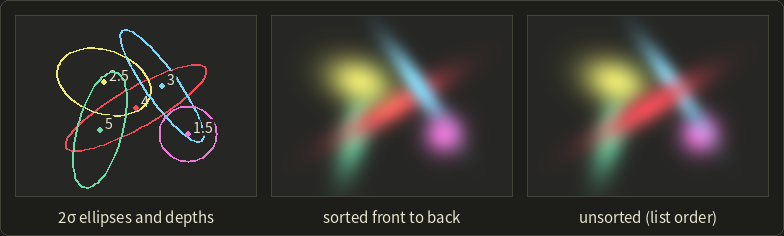
The tile rasterizer
3DGS doesn't use the triangle rasterizer; it has its own, in compute:
- Project every Gaussian, compute , its color for the view direction from the spherical harmonics, and the screen rectangle it covers.
- Duplicate each splat once per 16 × 16-pixel tile it touches, with a 64-bit key: the tile index in the upper bits and the depth in the lower 32 bits.
- Sort all keys with one GPU radix sort; now every tile's splats are contiguous and in depth order.
- One workgroup per tile walks its list front to back and stops each pixel once its accumulated opacity reaches 0.9999.
Worked example. The splat above, centered at pixel with a 12-pixel radius, covers from 88 to 112 and from 48 to 72, which are tiles 5 to 7 in (, ) and 3 to 4 in : 6 key entries.
Sorting per tile instead of per pixel is an approximation (two splats can swap order inside a tile), one source of the "popping" when the camera turns.
Training
Training starts from the sparse point cloud that structure from motion (SfM, chapter 17) produced while it estimated the camera poses, with one Gaussian per point.
Like NeRF, it renders the training views, compares them with the photos and backpropagates into every parameter of every Gaussian, through the differentiable tile rasterizer.
Every 100 steps, adaptive density control (適応的密度制御) clones small Gaussians in under-reconstructed regions, splits large ones that cover too much detail, and removes nearly transparent ones; the paper trains for 30,000 steps.
The result is an explicit, editable set of primitives that rasterizes in real time, with large files, artifacts in views far from the photos and baked-in lighting as its weaknesses; at the time of writing, compression, anti-aliasing, relighting and engine support are active topics.
29.11 Neural textures, materials and generative models
Neural textures and materials
Neural textures (ニューラルテクスチャ; Thies, Zollhöfer and Nießner, "Deferred Neural Rendering: Image Synthesis using Neural Textures", ACM Transactions on Graphics, SIGGRAPH 2019) keep a mesh with UVs but store learned feature vectors in its texture instead of colors.
Rasterizing the mesh gives a screen-space image of features, which a network (a U-Net) turns into the final picture: deferred shading with a learned shader.
More recent work uses small networks inside the shader for neural materials: NVIDIA researchers (Zeltner and colleagues, 2024) replaced layered production materials with networks evaluated in real time, and neural texture compression (Vaidyanathan and colleagues, 2023) stores a material's texture stack as a compact latent texture plus a decoder, at a higher compression ratio than block formats (chapter 27) for similar quality.
The shader matrix operations of section 29.6 exist so that such small networks can run in ordinary pixel shaders.
Generative models
A generative model learns the distribution of its training data and draws new samples from it.
The dominant image generators at the time of writing are diffusion models (拡散モデル; Sohl-Dickstein and colleagues, 2015; Ho, Jain and Abbeel, 2020).
Training adds Gaussian noise to a clean image at a random noise level, , and teaches a network to predict the noise; generation starts from pure noise and removes predicted noise in a few dozen steps, guided by a text prompt or an image.
Worked example. With , a pixel and noise give ; if the network predicts exactly, , the clean value.
Running the process on a compressed latent image instead of pixels (latent diffusion, Rombach and colleagues, 2022) made it practical on consumer GPUs.
In CG production they already make concept art, textures, skies and backgrounds, and they reach into 3D: DreamFusion (Poole and colleagues, 2022) optimizes a NeRF until a diffusion model finds its renders plausible.
They also raise the legal questions of section 18.7.
Under the Japanese guidance described there, training on works is in general permitted as a non-enjoyment use, with exceptions; a generated output infringes when it is similar to an existing work and relied on it, as with any other copy; and material generated autonomously by an AI isn't a work, while a person's creative contribution can be.
In practice: check the license of the model and its outputs, don't prompt for a particular artist's or work's expression, review outputs for similarity before use, and record what was generated; the law differs between countries and is still developing at the time of writing.
29.12 What to learn next, and a look back at Part 2
Part 2 in one table
Part 1 gave you every keyword of the exam syllabus; Part 2 opened up the techniques behind them.
Here are the tools it added:
| Chapter | Topic | Key tools |
|---|---|---|
| 19 | projection and rasterization | projection for any depth convention, reversed Z, edge functions |
| 20 | anti-aliasing and transparency | SSAA, MSAA, TAA; order-independent transparency |
| 21 | mesh processing and SDFs | QEM simplification, baking, sphere tracing |
| 22 | physically based shading | microfacet BRDFs, metallic–roughness, IBL |
| 23 | Monte Carlo rendering | importance sampling, MIS, path tracing, denoising |
| 24 | real-time shadows, AO, GI | cascades, PCSS, GTAO, probes, ReSTIR |
| 25 | character animation | dual quaternions, motion matching, full-body IK |
| 26 | physics simulation | implicit integration, contacts, XPBD, fluids |
| 27 | HDR and image processing | tone mapping, PQ and HLG, frequency-domain filters |
| 28 | volumes and advanced NPR | participating media, stylized characters and lines |
| 29 | GPU systems and neural rendering | occupancy, GPU-driven rendering, NeRF, splatting |
A theme runs through all of them: a rendering technique is an estimate of an integral (over a pixel, over directions, along a ray, over time), and each chapter chose where to put the samples, how to reuse them, and what error to accept.
NeRF and 3DGS are the latest example: the volume rendering integral of chapter 28, sampled the way chapter 23 taught, blended the way chapter 20 taught, and fitted to photos with gradient descent.
What to learn next
- Write the code. The GLSL series and the OpenGL series of this site come next in the learning order; most worked examples of this series become a shader or a small program there.
- Then an explicit API. Once OpenGL is comfortable, Vulkan, Direct3D 12 or Metal teach you the command buffers, barriers and GPU-driven techniques of sections 29.2 and 29.3 by doing.
- Read the classics. Real-Time Rendering (Akenine-Möller and colleagues), Physically Based Rendering (Pharr, Jakob and Humphreys, free online), and SIGGRAPH, HPG and EGSR course notes.
- Learn a little machine learning. A small NeRF or splatting trainer touches cameras, sampling, compositing and optimization at once; and read every "at the time of writing" here as an invitation to check what has changed.
Next: the mini-exam
The next chapter is a mini-exam of 40 questions in the style of the CG Engineer Certification, Expert level: chapter 30.
It covers the exam syllabus, that is Part 1 (chapters 2 to 18), not the Part 2 material of this chapter; chapter 31 gives its answers and explanations, together with the answers to every multiple-choice question in the chapters, this one included.
Review the "Exam points" lists and key-terms tables of Part 1 before you start.
29.13 Summary
- Occupancy is limited by registers, shared memory and a warp maximum; resident warps hide memory latency, . Compute shaders cooperate through shared memory; async compute overlaps queues.
- Explicit APIs record command buffers on many threads, compile pipeline state in advance and leave barriers and descriptors (bindless) to the application.
- Mesh shaders process meshlets; GPU-driven renderers cull on the GPU (frustum, two-phase Hi-Z) and draw indirectly; virtualized geometry picks cluster LODs by on-screen error; virtual texturing streams pages.
- Hardware ray tracing: a TLAS of instances over BLASes of triangles, shaders chosen through the shader binding table, inline ray queries. VRS and clustered shading spend shading work where it shows.
- Neural networks are matrix–vector products with nonlinearities, trained by gradient descent and backpropagation. Neural upscalers learn TAA's history decisions; frame generation adds smoothness, not responsiveness.
- NeRF: , , , trained by rendering, with positional encoding and hierarchical sampling; Instant-NGP moves the storage into multiresolution hash grids.
- 3D Gaussian splatting: , , tile-sorted front-to-back blending, adaptive density control. Neural textures put networks into shading; diffusion models generate content, with chapter 18's caveats.
29.14 Key terms
| English | 日本語 |
|---|---|
| occupancy | 占有率(オキュパンシー) |
| latency hiding | レイテンシ隠蔽 |
| register, shared memory (LDS) | レジスタ、共有メモリ(LDS) |
| compute shader, workgroup | コンピュートシェーダー、ワークグループ |
| async compute | 非同期コンピュート |
| explicit API | 明示的なAPI |
| command buffer | コマンドバッファ |
| pipeline state object (PSO) | パイプラインステートオブジェクト(PSO) |
| barrier | バリア |
| descriptor, bindless | デスクリプタ、バインドレス |
| mesh shader, task shader | メッシュシェーダー、タスクシェーダー |
| meshlet | メッシュレット |
| GPU-driven rendering | GPU駆動レンダリング |
| indirect draw | インダイレクト描画 |
| hierarchical Z | 階層Z(Hi-Z) |
| virtualized geometry | 仮想化ジオメトリ |
| visibility buffer | ビジビリティバッファ |
| virtual texturing | 仮想テクスチャ |
| BLAS, TLAS | ボトムレベル加速構造(BLAS)、トップレベル加速構造(TLAS) |
| shader binding table (SBT) | シェーダーバインディングテーブル(SBT) |
| ray generation, closest-hit, any-hit, miss shader | レイ生成シェーダー、最近接ヒットシェーダー、任意ヒットシェーダー、ミスシェーダー |
| ray query | レイクエリ |
| variable rate shading (VRS) | 可変レートシェーディング(VRS) |
| tiled forward (Forward+), clustered shading | タイルドフォワード(Forward+)、クラスタードシェーディング |
| neural network, multilayer perceptron (MLP) | ニューラルネットワーク、多層パーセプトロン(MLP) |
| activation function, loss function | 活性化関数、損失関数 |
| gradient descent, backpropagation | 勾配降下法、誤差逆伝播法 |
| training, inference | 学習、推論 |
| temporal upscaling, super-resolution | 時間方向アップスケーリング、超解像 |
| frame generation | フレーム生成 |
| neural radiance field (NeRF) | ニューラル放射輝度場(NeRF) |
| volume density, transmittance | 体積密度、透過率 |
| positional encoding, spectral bias | 位置エンコーディング、スペクトルバイアス |
| hierarchical sampling | 階層的サンプリング |
| multiresolution hash encoding | 多重解像度ハッシュエンコーディング |
| 3D Gaussian splatting (3DGS), splat | 3Dガウシアンスプラッティング(3DGS)、スプラット |
| covariance matrix, Jacobian | 共分散行列、ヤコビ行列 |
| adaptive density control | 適応的密度制御 |
| neural texture | ニューラルテクスチャ |
| diffusion model | 拡散モデル |
29.15 Challenges
- ★ For the example block of section 29.1 (65,536 registers, at most 48 warps, 4 schedulers, 100 KB of shared memory), compute the occupancy of a shader with 96 registers per thread. Then a compute workgroup of 128 threads uses 48 registers per thread and 20 KB of shared memory: how many workgroups fit, which resource limits them, and what is for , ?
- ★ An upscaler outputs 2560 × 1440. Compute the render resolution and the fraction of pixels for Quality (1.5), Balanced (1.7) and Performance (2.0), and the jitter sequence length for each. If a native frame takes 14 ms of which 12 ms scale with the pixels, and the upscaler costs 1 ms, how long does a Performance frame take?
- ★★ A NeRF ray has four samples with and , colors 0, 0.9, 0.5, 0.2 (one channel) and background 1. Compute every , and , the pixel value and the expected depth (samples at ). How many of 64 fine samples would hierarchical sampling put near each sample?
- ★★ A spherical Gaussian with (standard deviation 1 cm) is at view-space position m, seen by a camera with pixels. Compute , and the two standard deviations on screen. Why is the splat no longer round, and in which direction is it stretched?
- ★★★ An Instant-NGP level has resolution 153 and a table of entries. How many grid vertices share one entry on average? Explain why training still works without resolving collisions, and why helps the cache. What would go wrong if every level were hashed into one shared table?
Multiple choice
Q1 ★ Which of the following statements about modern GPU architecture is correct?
| A | Each lane of a warp fetches and decodes its own instruction stream, so a divergent branch costs nothing extra. |
| B | Higher occupancy always makes a shader faster, so the number of registers per thread should be minimized at any cost. |
| C | Shared memory (LDS) is visible to every workgroup on the GPU and is mainly used to pass data from one frame to the next. |
| D | When a shader needs more registers per thread, fewer warps can be resident on a block, so the GPU has fewer warps to switch to while others wait for memory. |
| E | Async compute runs compute shaders on the CPU while the GPU draws the frame. |
Q2 ★★ Which of the following statements about hardware ray tracing and GPU-driven rendering is correct?
| A | The BLAS holds the instances with their transforms, and the TLAS holds the triangles of each mesh in object space. |
| B | Drawing 10,000 copies of a tree with ray tracing requires 10,000 BLASes, each with its own copy of the triangles. |
| C | A ray query lets an ordinary shader, such as a compute or fragment shader, trace a ray inline and examine the result itself, without the shader binding table of the ray tracing pipeline. |
| D | A mesh shader is run once per vertex by the fixed-function input assembler, exactly like a vertex shader. |
| E | In GPU-driven rendering the CPU tests every object's bounding sphere against the frustum and records one draw command per visible object. |
Q3 ★★ Which of the following statements about neural rendering is correct?
| A | NeRF stores the scene as millions of explicit 3D Gaussians and draws them with a tile rasterizer. |
| B | Positional encoding removes high frequencies from the input so that the network learns a smoother function. |
| C | 3D Gaussian splatting needs no sorting, because alpha blending gives the same result in any order. |
| D | Frame generation samples the player's input for every generated frame, so it reduces input latency as much as rendering at the higher frame rate would. |
| E | In NeRF's volume rendering, a sample's weight is its alpha times the transmittance of everything in front of it, so a sample behind an almost opaque surface contributes almost nothing. |
29.16 Practical assignment
Run a GPU, a NeRF and a Gaussian splat on paper: plan the occupancy of three shaders, composite one ray of a radiance field, and draw and blend a splat on graph paper.
You need graph paper (5 mm squares), a ruler, a protractor, a pencil, three colored pens and a calculator with .
Part A: warps and latency.
Use the example block of section 29.1: 65,536 registers, at most 48 warps of 32 threads, 4 schedulers with 12 slots each.
- Compute the resident warps and the occupancy for shaders with 24, 56 and 100 registers per thread.
- Draw three grids of 4 × 12 squares, one per shader, and color the resident warps like the occupancy figure, spreading them evenly over the four schedulers.
- Latency. Each warp issues cycles of work and then waits cycles. Compute how many warps per scheduler full hiding needs, and for each of the three shaders.
Part B: one ray of a radiance field.
Five samples at have and brightness values (one channel); the background is 1.
- Compute , and in a table (four decimals), then the pixel value and the depth .
- Draw a bar chart like the NeRF figure: as outlined bars, as filled bars, and as a step line (1 cm = 0.1 on the vertical axis).
- Resample. Split 32 fine samples among the five samples in proportion to their normalized weights, rounding to whole numbers that add up to 32.
Part C: one splat on graph paper.
A splat has its center at the origin of your paper, standard deviations 3 and 1 pixels along axes rotated by 45°, and opacity 0.9; let one square be one pixel, to the right and up.
- Covariance. Compute for a 45° rotation, its determinant and its inverse.
- Draw the 2σ ellipse: semi-axes 6 and 2, the long one along the 45° line. Mark the pixels , , and .
- Evaluate at the four pixels with the formula of section 29.10. Which is largest, and why does get much less than at the same distance?
- Blend. A second splat, isotropic with standard deviation 2 pixels, opacity 0.6 and center , lies in front. At pixel compute its , then blend blue (front splat) and red (your first splat) over white, front to back. Repeat in the wrong order.
How to check yourself:
- Part A: the three shaders give 48, 36 and 20 warps; full hiding needs warps per scheduler, so the first shader hides all latency and the others reach about 82% and 45%.
- Part B: the transmittance at the end must equal , and the weights plus that value must add up to 1; the largest weight belongs to the third sample, and the depth comes out a little below 1.8.
- Part C: has 5 on the diagonal and 4 off it, and its determinant is ; lies on the long axis and gets the largest (about 0.81), the smallest.
- Part C: both blending orders leave the same transmittance (about 0.13), because is a product; only the color changes, and the blue channel in the correct order is more than twice the one in the wrong order (about 0.45 against 0.19).
コメント(0)
まだコメントはありません。
ログインするとコメント出来ます。