7. Matrix Multiplication and the Transpose
In chapter 6 a matrix took a vector and gave back a new vector.
But in a real game we almost never apply just one transformation.
A character is scaled, then rotated, then placed in the world, then seen by a camera, then projected onto the screen.
That's at least four or five matrices for every single vertex.
In this chapter we learn how to multiply two matrices together, so that a whole chain of transformations collapses into one matrix.
We'll also see why the order matters so much, and meet the transpose, a simple flip that you need to read other people's formulas, books and shader code.
7.1 The idea: doing one thing after another
Say we have two matrices, and .
We want to transform a vector with first, and then transform the result with :
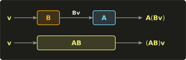
That's two matrix–vector multiplications.
For one vertex, fine.
For a million vertices, every frame, through five matrices, it starts to hurt.
Wouldn't it be nice to have a single matrix that does both jobs at once, so that for every ?
That matrix exists, and it's called the product .
Look at the order: we write , but happens first, because it's the one standing right next to the vector.
Matrix products are read right to left.
7.2 What the formula is
For two matrices and , the element in row and column of the product is the dot product of row i of A with column j of B:
For 2 × 2 matrices, written out completely:
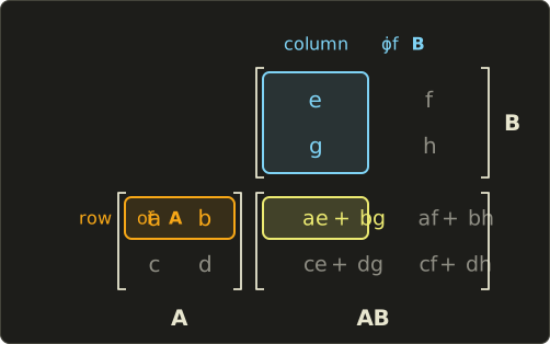
The size rule is the same as in chapter 6, just with more columns on the right:
The inner numbers must match (each row of must be as long as each column of ), and the outer numbers give the size of the result.
So a 2 × 3 matrix times a 3 × 2 matrix is a 2 × 2 matrix, but a 3 × 2 matrix times a 2 × 3 matrix is a 3 × 3 matrix.
A 3 × 2 times a 3 × 2 is simply not defined.
In graphics we nearly always multiply square matrices of the same size (4 × 4 times 4 × 4), so the rule is easy to satisfy.
7.3 How it works
Why row times column?
Here is the reasoning, using the key insight from chapter 6: the columns of a matrix are where the basis vectors land.
The product must send each basis vector to the same place as "first , then ".
sends the j-th basis vector to the j-th column of ; call that column .
Then sends to .
So the j-th column of the product has to be :
In words: to multiply two matrices, multiply the left matrix with each column of the right matrix.
And we already know how to compute from chapter 6: each component is a row of dotted with .
Row i of dotted with column j of : that's the formula.
Keep this "column by column" picture in mind, because it's exactly how our C++ code will do it.
A 2 × 2 example
Let's multiply these two:
There are four elements to compute, one for each combination of a row of and a column of .
- Row 1 of A is , column 1 of B is :
- Row 1 of A is , column 2 of B is :
- Row 2 of A is , column 1 of B is :
- Row 2 of A is , column 2 of B is :
Now the other way around, :
- Row 1 of B is , column 1 of A is :
- Row 1 of B is , column 2 of A is :
- Row 2 of B is , column 1 of A is :
- Row 2 of B is , column 2 of A is :
Completely different!
With ordinary numbers , but with matrices in general.
We say matrix multiplication is not commutative.
Section 7.4 shows what that means geometrically.
A 3 × 3 example
Let's reuse the matrix from chapter 6 as and pick a new :
Nine elements this time.
The rows of are , and .
The columns of are , and .
Row 1 of A with each column of B:
Row 2 of A with each column of B:
Row 3 of A with each column of B:
(If you compute you'll get , different again.)
Checking that it really is "B, then A"
The whole point of was that it does the same as applying and then .
Let's test that with .
The long way, first: with view 2 from chapter 6, is just the sum of the columns of :
Then , row by row:
The short way, with the product we computed (again just the sum of its columns, because ):
Same answer.
One matrix, one multiplication, same result as two.
7.4 Order matters
Why is different from ?
Because "do B, then A" is a different instruction from "do A, then B".
Putting on socks and then shoes is not the same as shoes and then socks.
Let's see it with two simple 2D transformations.
The first one stretches everything to twice its width:
Read the columns: lands on , stays at .
The second one is a quarter turn counter-clockwise, a rotation by 90°.
We don't have the general rotation formula yet (that's chapter 8), but we don't need it: we only need to know where and go.
Turning a quarter turn counter-clockwise makes it point up, to .
Turning a quarter turn makes it point left, to .
Those are the columns:
Now the two products.
means "stretch first, then rotate":
means "rotate first, then stretch":
Apply both to the unit square.
With , the corners , and go to , and .
With , they go to , and .
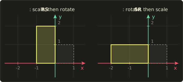
On the left, the square was first stretched into a wide 2 × 1 rectangle, then turned on its side: now it stands tall, 1 wide and 2 high.
On the right, the square was first turned (still a square), then stretched sideways: now it lies wide, 2 wide and 1 high.
Same two ingredients, different order, different result.
This is something you'll fight with in every 3D program you write.
In chapter 9 we'll build the model matrix , and you'll see what goes wrong when the order is mixed up.
The rule to remember: the matrix closest to the vector happens first.
7.5 Associativity and the identity
Order matters, but grouping doesn't.
For any three matrices of matching size:
This property is called associativity.
It makes sense: both sides mean "apply C, then B, then A", we're only choosing which two to glue together first.
The same is true with a vector at the end: , which is exactly what we checked numerically in section 7.3.
Associativity is the reason graphics is fast.
A vertex in a game goes through a chain like (projection, view, model, which we'll build in chapters 9 to 12).
Because of associativity, we're allowed to compute once, on the CPU, and then use that single matrix for every vertex.
Let's count the work.
A 4 × 4 times 4 × 4 product has 16 elements, each a dot product of length 4: that's multiplications and additions.
A 4 × 4 matrix times a 4D vector is 16 multiplications and 12 additions.
For a mesh with one million vertices:
| Method | Multiplications |
|---|---|
| for every vertex | |
| once, then one product per vertex |
Three times less work, for free, just because we're allowed to move the brackets.
And just like the number 1, the identity matrix leaves any matrix unchanged from either side:
"Do nothing, then A" is the same as "A, then do nothing", which is the same as "A".
7.6 The transpose
The transpose of a matrix flips it over its main diagonal: rows become columns and columns become rows.
We write it with a small T: .
The first row became the first column, the second row became the second column.
A 2 × 3 matrix becomes a 3 × 2 matrix.
The diagonal elements ( and here) stay where they are.
Transposing twice gets you back where you started: .
A column vector transposed becomes a row vector, a 1 × n matrix:
Remember section 6.5: if one side stores a matrix row-major and the other side reads it as column-major, the reader sees exactly the transpose.
That's one place you'll meet it in practice.
The transpose of a product
Here is the rule that matters most:
The transpose of a product is the product of the transposes in reverse order.
Let's check it with and from the 2 × 2 example.
We know , so .
The other side:
It matches.
Why the reverse order?
Element of is element of , which is row j of A dotted with column i of B.
Row j of A is column j of , and column i of B is row i of , so it's also row i of dotted with column j of : element of .
The dot product doesn't care which side is which, so the two are equal.
Reading other people's formulas: the row-vector convention
In this series vectors are columns and matrices stand on the left: .
That's the convention of OpenGL, GLSL, most math books and many engines (Unreal and DirectXMath use row vectors instead).
But a lot of code and books use the opposite: vectors are rows and matrices stand on the right, .
Old DirectX (the D3DX math library), much HLSL code, and several well-known graphics books do this.
Neither is wrong, but you have to be able to translate.
Transpose both sides of our formula and use the reverse-order rule:
So their matrix is simply our matrix transposed: .
A quick check with from before and :
Same numbers, one written standing up and one lying down.
Two practical consequences:
- Chains reverse. Our (scale first) becomes in row-vector style. That's why DirectX-style code reads left to right: "v times scale times rotation times translation".
- Printed matrices are flipped. When a row-vector book shows a matrix, it's the transpose of the one we'd write. For example, the translation numbers that we'll put in the last column (chapter 9) appear in their last row.
There's a nice coincidence hiding here.
Row-vector matrices are our matrices transposed, and row-major storage is column-major storage transposed.
Two flips cancel out, so a row-major, row-vector matrix (DirectX style) has exactly the same bytes in memory as a column-major, column-vector matrix (OpenGL style).
In shaders
All three shading languages let you multiply on either side:
- In Slang and HLSL,
mul(M, v)treatsvas a column, andmul(v, M)treatsvas a row. Somul(v, M)gives the same asmul(transpose(M), v). - In GLSL,
m * vtreatsvas a column, andv * mtreatsvas a row. Sov * mgives the same astranspose(m) * v. - All three languages have a built-in
transpose()function.
So if you copy a shader that writes mul(position, worldViewProj), it expects the matrix in the row-vector convention.
Either upload the transpose, or swap the arguments.
And remember chapter 6: in Slang and HLSL, the matrix–matrix product is mul(A, B) too, never A * B.
7.7 Use in graphics programming
The model–view–projection chain
Every 3D vertex shader you'll write does some version of this:
- is the model matrix: it places the object in the world (chapter 9).
- is the view matrix: it moves the world so that the camera sits at the origin (chapter 11).
- is the projection matrix: it squashes the visible part of the world into the box the GPU draws (chapter 12).
Read right to left: model first, then view, then projection.
Here's a vertex shader that receives the three matrices separately and applies them.
Look at the brackets: we apply the matrices to the vector one at a time, which is three matrix–vector products.
struct Matrices {
  float4x4 model;
  float4x4 view;
  float4x4 proj;
};

ConstantBuffer<Matrices> matrices;

struct VertexOutput {
  float4 position : SV_Position;
};

[shader("vertex")]
VertexOutput vertexMain(float3 position : POSITION) {
  VertexOutput output;
  float4 world = mul(matrices.model, float4(position, 1.0));
  float4 viewPos = mul(matrices.view, world);
  output.position = mul(matrices.proj, viewPos);
  return output;
}
#version 450
layout(set = 0, binding = 0) uniform Matrices {
mat4 model;
mat4 view;
mat4 proj;
};
layout(location = 0) in vec3 position;
void main() {
gl_Position = proj * (view * (model * vec4(position, 1.0)));
}struct Matrices {
float4x4 model;
float4x4 view;
float4x4 proj;
};
ConstantBuffer<Matrices> matrices;
struct VertexOutput {
float4 position : SV_Position;
};
VertexOutput vertexMain(float3 position : POSITION) {
VertexOutput output;
float4 world = mul(matrices.model, float4(position, 1.0));
float4 viewPos = mul(matrices.view, world);
output.position = mul(matrices.proj, viewPos);
return output;
}
Why the extra brackets in GLSL?
* is evaluated left to right, so proj * view * model * v means ((proj * view) * model) * v: two full matrix–matrix products (128 multiplications) for every vertex, before the actual transform.
With the brackets, it's three matrix–vector products (48 multiplications).
Associativity guarantees the same result, but the cost is very different.
The best option is to do once on the CPU and upload just one matrix, like the mvp shader from chapter 6.
Engines often keep model separate (lighting needs world positions) and combine only proj * view into one view-projection matrix per frame.
Scene graphs and hierarchies
Things in games are attached to other things.
A sword is held in a hand, the hand is at the end of a forearm, the forearm hangs from an upper arm, the upper arm is attached to the body.
When the body turns, everything attached should turn with it.
The trick is that each part only stores its local matrix: how it's placed relative to its parent.
Its matrix in the world is its parent's world matrix times its own local matrix:

Expanded, the sword's world matrix is .
Right to left again: first the sword is placed in the hand, then the hand on the forearm, and so on, up to the body in the world.
In C++ it's just a loop down the tree:
// Each frame, from the root down to the leaves.
Mat4 upperWorld = bodyWorld * upperLocal;
Mat4 foreWorld  = upperWorld * foreLocal;
Mat4 handWorld  = foreWorld * handLocal;
Mat4 swordWorld = handWorld * swordLocal;
Animate foreLocal (bend the elbow) and the hand and sword follow automatically, because they're computed from foreWorld.
Real local matrices also contain a position offset (the forearm starts at the end of the upper arm), which needs translation from chapter 9, but the multiplication chain is exactly this.
Unity's Transform, Godot's Node3D, Unreal's scene components and glTF's node hierarchy all work this way.
CPU or GPU?
A good rule of thumb:
- Things that are the same for every vertex of a draw call (model, view, projection, a parent chain) are multiplied together on the CPU, once per frame or once per object.
- Things that are different per vertex are done on the GPU: one matrix–vector product per vertex.
A small exception is skeletal animation, where each vertex blends a few bone matrices.
Even there, the bone matrices themselves (each a long chain like the sword above) are combined on the CPU or in a compute pass, and the vertex shader only does a few matrix–vector products.
7.8 Other uses
Robotics
A robot arm is the same as our sword hierarchy.
Each joint has a matrix that depends on its angle, and the position of the gripper is the product of all of them, .
Computing this is called forward kinematics, and it's literally a chain of matrix products.
Counting paths in a graph
Take a little one-way road network: A to B, A to C, B to C and C to A.
Write a 1 in row i, column j if there's a road from i to j:
Element of is , which counts the stops k where you can go i to k and then k to j.
So counts routes with exactly two roads.
Row A says: from A you can reach A in two steps (A, C, A) and C in two steps (A, B, C), but not B.
counts three-road routes, and so on.
Social networks, web crawlers and route planners use this idea.
Neural networks
A layer of a neural network takes an input vector and computes , where is a matrix of learned weights (plus an offset, which we'll ignore here).
Two layers in a row are .
By associativity, that's just one layer with the matrix !
This is exactly why neural networks put a non-linear function (like "replace negative numbers with 0") between the layers: without it, a hundred layers would be no more powerful than one.
Training and running these networks is mostly huge matrix products, and that's why GPUs, built for graphics, became the machines for AI.
Markov chains, many steps at once
In chapter 6, the weather matrix took us from today to tomorrow, and we applied it twice to get the day after.
With matrix products we can jump two days at once:
The first column is exactly what we got in chapter 6 for "sunny today, two days from now".
tells you the weather a month from now.
7.9 Code
Here is matrix times matrix, exactly as in linalg.hh:
// 行列×行列 / matrix × matrix (chapter 7)
inline Mat4 operator*(const Mat4 &a, const Mat4 &b) {
  Mat4 r;
  for (int i = 0; i < 4; ++i) r.c[i] = a * b.c[i];
  return r;
}
That's the "column by column" picture from section 7.3: column i of the result is a times column i of b.
It reuses the matrix–vector operator* from chapter 6, so we don't need to write out a single dot product.
And the transpose:
// 転置 / transpose (chapter 7)
inline Mat4 transpose(const Mat4 &m) {
  Mat4 r;
  for (int row = 0; row < 4; ++row)
    for (int col = 0; col < 4; ++col)
      r.at(row, col) = m.at(col, row);
  return r;
}
This is the definition written as code.
The at() accessor from chapter 6 keeps us from having to think about the column-major memory at all.
A test program
We'll put the 2 × 2 matrices from section 7.3 into the top-left corner of 4 × 4 identity matrices, and check the products, the transpose and associativity.
The printVec4 and printMat4 helpers are the same as in chapter 6.
#include "linalg.hh"
#include <cstdio>

void printVec4(const char *name, Vec4 v) {
  printf("%s = (%g, %g, %g, %g)\n", name, v.x, v.y, v.z, v.w);
}

void printMat4(const char *name, const Mat4 &m) {
  printf("%s =\n", name);
  for (int row = 0; row < 4; ++row) {
    printf("  [%6g %6g %6g %6g ]\n", m.at(row, 0), m.at(row, 1), m.at(row, 2), m.at(row, 3));
  }
}

int main() {
  // A and B from section 7.3, in the top-left corner of a 4x4 identity.
  Mat4 a = Mat4::identity();
  a.at(0, 0) = 1; a.at(0, 1) = 2;
  a.at(1, 0) = 3; a.at(1, 1) = 4;

  Mat4 b = Mat4::identity();
  b.at(0, 0) = 5; b.at(0, 1) = 6;
  b.at(1, 0) = 7; b.at(1, 1) = 8;

  printMat4("a * b", a * b);
  printMat4("b * a", b * a);
  printMat4("transpose(a)", transpose(a));

  // Composition: (a * b) * v gives the same as a * (b * v).
  Vec4 v = {1, 1, 0, 1};
  printVec4("(a * b) * v", (a * b) * v);
  printVec4("a * (b * v)", a * (b * v));
  return 0;
}
Expected output:
a * b =
  [    19     22      0      0 ]
  [    43     50      0      0 ]
  [     0      0      1      0 ]
  [     0      0      0      1 ]
b * a =
  [    23     34      0      0 ]
  [    31     46      0      0 ]
  [     0      0      1      0 ]
  [     0      0      0      1 ]
transpose(a) =
  [     1      3      0      0 ]
  [     2      4      0      0 ]
  [     0      0      1      0 ]
  [     0      0      0      1 ]
(a * b) * v = (41, 93, 0, 1)
a * (b * v) = (41, 93, 0, 1)
The top-left corners are exactly our hand-computed and .
The rest stays identity, because identity blocks multiply into identity blocks.
For the last two lines: applied to is , and doing then step by step gives the same.
7.10 Summary
- The product is one matrix that does "first B, then A". Products are read right to left.
- Element of is row i of A dotted with column j of B. Equivalently, column j of is A times column j of B.
- Sizes: (m × n) times (n × p) gives (m × p). The inner numbers must match.
- Matrix multiplication is not commutative: in general. Scale-then-rotate is not rotate-then-scale.
- It is associative: . That's why we can precompute one matrix for a million vertices.
- The identity changes nothing from either side: .
- The transpose swaps rows and columns, and .
- The row-vector convention (, DirectX style) uses transposed matrices and reversed chains. In Slang and HLSL
mul(v, M)equalsmul(transpose(M), v). - In graphics: the P V M chain, scene graphs (), and combining on the CPU what's shared by every vertex.
7.11 Challenges
- ★ Compute , then compute the same two matrices in the other order and confirm the answers differ.
- ★ Which of these products are defined, and what size is the result? (2 × 3)(3 × 4), (3 × 2)(3 × 2), (1 × 3)(3 × 1), (3 × 1)(1 × 3).
- ★ For and , compute and and check that they're equal. Then compute and see that it's not.
- ★ Using the 90° rotation from section 7.4, compute . Where do i and j land? What single rotation is that?
- ★★ Build the 90° rotation about the z axis as a
Mat4by setting its columns (c[0] = {0, 1, 0, 0},c[1] = {-1, 0, 0, 0}, the rest identity). Printr * r * r * r; you should get the identity. Then make a scaleswiths.at(0, 0) = 2and print(r * s) * Vec4{1, 0, 0, 0}and(s * r) * Vec4{1, 0, 0, 0}; you should get(0, 2, 0, 0)and(0, 1, 0, 0). - ★★ Write
Vec4 mulRow(Vec4 v, const Mat4 &m)that treatsvas a row vector (component j of the result isvdotted with column j ofm). Test it with the matrix from the chapter 6 test program andv = {2, 1, 3, 1}: you should get(14, 5, 6, 1), andtranspose(m) * vshould print the same. - ★★★ A DirectX-era book writes a vertex transform as with row vectors, where the subscript b marks the book's matrices. Rewrite it in this series' convention using our matrices , , , explain why the order of the letters flips, and explain why the bytes in memory can still be identical between the two styles.
コメント(0)
まだコメントはありません。
ログインするとコメント出来ます。