26. Physics Simulation
Chapter 14 gave you the toolbox of physics-based animation: explicit and semi-implicit Euler, Verlet and Runge–Kutta, the spring that explodes, mass–spring cloth, rigid bodies with torque and the inertia tensor, broad and narrow phase, restitution and impulses, grids versus particles for fluids.
It named most of the methods that real engines use and stopped there.
This chapter opens them up.
We'll solve a stiff spring with implicit Euler and see why it never explodes; make rigid bodies tumble correctly, find box contacts with the separating axis test and resolve them with impulses and friction the way game engines do; then switch to position-based dynamics and XPBD, the method behind most real-time cloth.
For fluids we'll read the Navier–Stokes equations term by term, run Stable Fluids on a 2×2 grid by hand, compute an SPH density, and compare PIC, FLIP, APIC and MPM.
We'll end with hair, destruction, GPU physics and determinism.
This is Part 2, beyond the exam syllabus, but it grows directly out of the syllabus item physics-based animation (物理ベースアニメーション) of chapter 14, and the exam points at the end of section 26.5 say where it ties back.
Characters, skinning and ragdolls are chapter 25; rendering smoke and fire as participating media is chapter 28.
The math is the Linear Algebra series: the dot and cross products (chapters 4 and 5), matrix products and the transpose (chapter 7), inverses (chapter 10) and quaternions (chapter 13).
26.1 Time integration revisited
Stiffness
Section 14.2 ended with three escape routes from the exploding spring: smaller steps, damping, and implicit integration.
A simulation is stiff (硬い, スティッフ) when it contains motions on very different time scales: cloth that barely stretches (stretch vibrations of a few milliseconds) but swings slowly (seconds), a car suspension, a stack of heavy boxes.
An explicit method must resolve the fastest motion even when nobody can see it, so the stiffest spring in the scene dictates the time step for everything.
Take the spring of section 14.2 with N/m and kg, so rad/s and the period is s.
Semi-implicit Euler needs , that is s.
At s it explodes: goes 1, −5.25, 21.3, −85.3, 341.3.
A 10 g cloth particle on the same spring has rad/s and needs s; real fabric is much stiffer still.
Implicit Euler, worked
The implicit Euler method (陰的オイラー法, also 後退オイラー法, backward Euler) evaluates everything at the end of the step:
The unknowns appear on both sides, so each step means solving equations.
For one linear spring we can do it by hand: substitute the first equation into the second,
Worked example.
, , , , so and .
- Step 1: , .
- Step 2: , .
Check step 1 with the first equation: .
The energy starts at 50 J and is J after one step: exactly .
Every step divides the energy by , the mirror image of explicit Euler, which multiplies it by the same number (section 14.2).
So implicit Euler can't explode, whatever the step.
The price is visible in the picture: it loses energy that the real spring keeps.
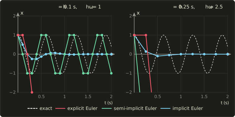
At s () the energy halves every step, so after one second ( steps) only of it is left: the spring has stopped although it should swing forever.
At a 60 Hz step the loss is per step, still after one second.
For cloth this artificial damping is often welcome (fabric is damped anyway); for a pendulum or an orbit it's wrong.
That's the trade: stable, but numerically damped (数値減衰).
Stability regions
Why does one method always grow and the other always shrink?
Numerical analysts study every integrator on the test equation (テスト方程式)
with a complex number .
Its solution decays for negative real part and oscillates for imaginary .
Applying a method gives with , and the method is stable when .
The set of such is the method's stability region (安定領域).
- Explicit Euler: , so . Stable inside the disk of radius 1 around .
- Implicit Euler: , so . Stable outside the disk of radius 1 around , which includes the whole left half-plane. A method with that property is called A-stable (A安定).
A spring with no damping behaves like two test equations with (the eigenvalues of the 2×2 matrix that maps to ).
Then lies on the imaginary axis, and
Their squares are the energy factors we've seen; the imaginary axis touches the explicit disk only at 0, so explicit Euler is unstable for an undamped spring at every step size.
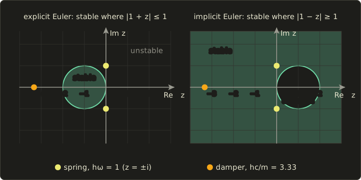
Damping is a real negative : a damper with N·s/m on 1 kg has , so at 60 Hz .
Explicit Euler multiplies the velocity by per step, a damper that adds energy (it would need s); implicit Euler multiplies it by , a calm decay.
(Semi-implicit Euler's step matrix for the spring has eigenvalues of length exactly 1 while : the bounded energy of section 14.2.)
The implicit midpoint rule (陰的中点法), , is stable on exactly the left half-plane and has on the imaginary axis: it keeps a linear spring's energy exactly, for the same solving cost.
Implicit integration in practice
A real scene has thousands of particles and nonlinear forces (a spring's force depends on the direction between its ends).
Then is a large nonlinear system, solved with Newton's method (ニュートン法): linearize the forces around the current state and solve the linear system, once or a few times.
Baraff and Witkin (1998, cited in section 14.2) take one Newton step per time step:
is the (diagonal) mass matrix, the stiffness matrix (剛性行列): how every force changes when every position moves a little.
For our 1D spring (, ) it gives , the same as above.
For a cloth, the matrix has one 3×3 block per spring end, so it's huge but sparse (疎), and it's solved iteratively with the conjugate gradient method (共役勾配法).
Film cloth and hair solvers work this way; games mostly use the cheaper position-based methods of section 26.3.
26.2 Rigid bodies in depth
The state, and the inertia tensor in world space
Section 14.5 gave a rigid body a position , a velocity , an orientation and an angular velocity , and related torque to angular acceleration through the inertia tensor (慣性テンソル) .
Two details make or break a rigid-body simulator.
First, is constant only in the body's own coordinates.
For a box of mass with side lengths , , along its local x, y, z axes, it's diagonal:
When the body rotates by the matrix , its inertia seen from the world changes:
(Read it right to left: rotate a world vector into body space, apply the body inertia, rotate back. The inverse is cheap because for a rotation, Linear Algebra chapter 10.)
Engines store once and rebuild every step.
Worked example.
A box of kg, m: kg·m².
Rotate it by 45° about z; with , the upper-left 2×2 block becomes
and is unchanged.
Now give it the angular momentum (角運動量) , a spin about the world x axis.
The angular velocity is ; the inverse of the 2×2 block is , so
The box doesn't spin about the axis you pushed it around: is 23° away from .
Only about the three principal axes (慣性主軸), the body's own x, y and z here, are and parallel.
That's why a thrown book wobbles.
Second, with changing, the rotational version of gets an extra term (Euler's equations):
The gyroscopic term (ジャイロ項) makes a spinning racket tumble.
It's quadratic in , and semi-implicit Euler can pump energy into it until a fast, elongated body blows up, so engines either drop it (stable but "too stable") or integrate it implicitly with one Newton step, as Erin Catto showed in his GDC 2015 talk on numerical methods.
Integrating the orientation
Section 14.5 updated the orientation quaternion with and renormalized it.
This is explicit Euler applied to the quaternion derivative , with in world space and the Hamilton product of Linear Algebra chapter 13.
Worked example.
Start at the identity (written ) and spin about z with rad/s for s.
, so .
Its length is ; normalized it's .
A unit quaternion rotates by , so this is rad, where the exact answer is rad.
The body spins 0.3% too slowly, and without the normalization the length would grow by 1.004988 per step.
The exact alternative is the exponential map: multiply from the left by the rotation by about , here .
Contact generation: the separating axis test
Chapter 14 named the narrow phase's job: find the contact points, the contact normal and the penetration depth.
For convex polygons and polyhedra the classic tool is the separating axis theorem (分離軸定理, SAT): two convex shapes don't overlap if and only if there is an axis on which their projections (their "shadows") don't overlap.
For polygons in 2D, it's enough to test the edge normals of both shapes; for boxes that means the two axes of each box.
Projecting a box with center , unit axes , and half-extents , onto a unit axis gives an interval centered at with the radius
and two boxes overlap on that axis by ; a negative value is a gap.
Worked example.
Box A sits at the origin, axis-aligned, with half-extents .
Box B has half-extents and is rotated so that its axes are and (an angle of about 36.9°).
On the four axes, A's radii are 2, 1, and ; B's are , , 1 and 0.5.
| Axis | B at (3, 1.8): distance, overlap | B at (2.5, 1.5): distance, overlap | ||
|---|---|---|---|---|
| 2 | 1.1 | 3, 0.1 | 2.5, 0.6 | |
| 1 | 1.0 | 1.8, 0.2 | 1.5, 0.5 | |
| 2.2 | 1 | 3.48, −0.28 | 2.9, 0.3 | |
| 2.0 | 0.5 | 0.36, 2.14 | 0.3, 2.2 |
With B centered at , the distance along is , more than : a gap of 0.28, so the boxes are separate, although they overlap on both of A's axes (which is all an AABB test would look at).
With B at , all four axes overlap, so the boxes collide.
The axis of smallest overlap is the contact normal, (pointing from A to B because ), and the overlap 0.3 is the penetration depth: moving B by separates them.
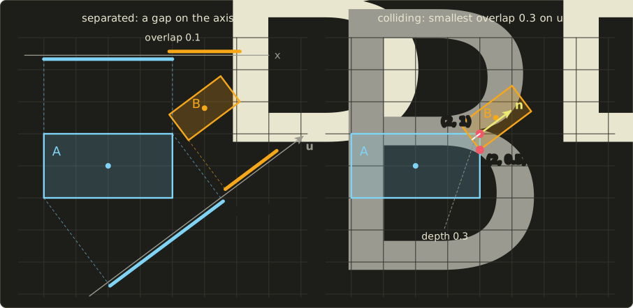
The normal and depth aren't enough for a box resting on a box: a single contact point would let it rock.
Engines build a contact manifold (接触点の集合, コンタクトマニフォールド) of up to 2 points in 2D (4 in 3D) by clipping.
The axis came from B, so the face of B facing A is the reference face (参照面), with outward normal .
The face of A most anti-parallel to it, A's right edge from to (its normal has the largest dot product with , 0.8), is the incident face (入射面).
Clip the incident edge to the side planes of the reference face, exactly like Sutherland–Hodgman clipping in chapter 6, section 6.3: in B's coordinates a point has , and the side plane cuts the edge at .
Keep the clipped points that lie behind the reference face: has , so it's deep; has , depth 0, just touching.
Two contact points, one deep and one touching: enough to keep B from rotating into A.
In 3D, two boxes have 15 candidate axes: 3 face normals of each box plus the 9 cross products of an edge of A with an edge of B (two edges can hit each other without any face being involved).
GJK and EPA
SAT needs the list of candidate axes, which is fine for boxes and convex polygons but not for spheres, capsules or arbitrary convex hulls.
The Gilbert–Johnson–Keerthi algorithm (GJK; Gilbert, Johnson and Keerthi, 1988) works with any convex shape that can answer one question, its support function (サポート関数): which point of the shape lies farthest in a given direction ?
For a sphere it's ; for a box, the corner on the side of .
The trick is the Minkowski difference (ミンコフスキー差) , the set of all differences of a point of A and a point of B.
A and B overlap exactly when some , that is, when the origin lies inside .
Its support function is , so we never build .
GJK grows a simplex (a point, a segment, a triangle, a tetrahedron) of support points of towards the origin; if it encloses the origin, the shapes overlap; if a support point can't get past the origin, they're separate and the closest simplex feature gives the distance.
When they overlap, the expanding polytope algorithm (EPA, van den Bergen, 2001) inflates the final simplex into a polytope until it finds the face of closest to the origin: its normal is the contact normal and its distance the penetration depth.
For our colliding boxes and : and , so reaches past the origin in that direction: the depth SAT found, which EPA finds as the minimum over all directions.
Contact constraints and impulses
Section 14.6 resolved a head-on collision with one impulse along the normal.
With rotation, the velocity that matters is the velocity of the contact point, , where is the offset from the center of mass to the contact.
A contact constraint (接触拘束) says that this point must not move into the other object, , and that the contact may push but never pull: the normal impulse .
An impulse along a direction at changes both velocities:
and so changes by with the effective mass (有効質量)
(plus the same terms for the second body when it isn't static).
To stop the approach completely (), apply .
Friction follows Coulomb's law (クーロン摩擦): the tangential impulse may be at most times the normal one, .
In 3D, the allowed contact impulses form the friction cone (摩擦円錐) around the normal, with half-angle ; engines usually approximate it with two tangent directions, a four-sided pyramid.
Inside the cone the contact sticks; on its surface it slides.
Worked example.
A crate (2D, a unit square with kg and kg·m²) falls with m/s onto a thin post that catches it under its bottom-right corner, , , , , .
In 2D the cross product is a number, here , and .
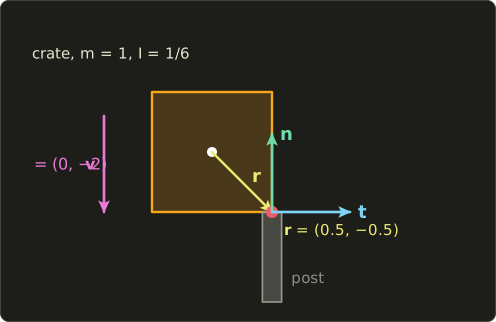
- Effective masses: for the normal, and the same for the tangent ().
- Normal: , so . Then and rad/s. The corner now has : stopped.
- Friction: the corner slides with m/s. Stopping it would need , but Coulomb allows only , so : the corner keeps sliding. Then and .
But now the corner moves into the post again: .
The friction impulse took away spin that the normal impulse relied on: solving one constraint broke the other, so we iterate.
Sequential impulses and projected Gauss–Seidel
Game engines visit the constraints one at a time, apply the impulse that fixes the current one, and sweep over all of them several times.
Erin Catto popularized it as sequential impulses (シーケンシャルインパルス) in his GDC talks ("Iterative Dynamics with Temporal Coherence", 2005; "Fast and Simple Physics using Sequential Impulses", 2006), the solver of Box2D.
Mathematically it's the projected Gauss–Seidel method (射影ガウス=ザイデル法, PGS): Gauss–Seidel iteration on the linear system of all contacts, with each unknown projected back into its allowed range after its update.
The key rule: keep an accumulated impulse per contact for the whole step and clamp the accumulated value, not each increment.
An increment may be negative (taking back some of an impulse that turned out too large); only the total must stay for the normal and inside for friction.
Continuing the crate:
| Iteration | total | total | after | ||
|---|---|---|---|---|---|
| 1 | 0.8 | −0.4 | (−0.4, −1.2) | 1.2 | −0.6 |
| 2 | 1.04 | −0.52 | (−0.52, −0.96) | 1.56 | −0.18 |
| 3 | 1.112 | −0.556 | (−0.556, −0.888) | 1.668 | −0.054 |
| 4 | 1.1336 | −0.5668 | (−0.5668, −0.8664) | 1.7004 | −0.0162 |
| exact | 8/7 ≈ 1.1429 | −4/7 ≈ −0.5714 | (−0.5714, −0.8571) | 12/7 ≈ 1.7143 | 0 |
The error shrinks by the factor 0.3 per iteration.
The exact answer comes from solving both conditions together: the contact slides, so ; then and gives .
The corner then slides at m/s to the right, and friction pushes left, as it should.
With many contacts convergence is slower (in a tall stack the top box's weight must travel down through every contact), so engines run a fixed number of iterations, typically 4 to 20, and accept the remaining error.
#include <algorithm>
#include <cstdio>
#include "linalg.hh"

// 2D cross products: r x n is a scalar, w x r is a vector.
float cross2(Vec2 a, Vec2 b) { return a.x * b.y - a.y * b.x; }
Vec2 crossW(float w, Vec2 r) { return {-w * r.y, w * r.x}; }

struct Body {
  float invMass, invInertia;
  Vec2 v;
  float w;  // angular velocity (rad/s, counter-clockwise)
};

// One contact point at offset r from the center, normal n, tangent t, against a static object.
struct Contact {
  Vec2 r, n, t;
  float mu;
  float Pn = 0.0f, Pt = 0.0f;  // accumulated impulses (keep them for warm starting)
};

void applyImpulse(Body &b, Vec2 r, Vec2 dir, float lambda) {
  b.v = b.v + (lambda * b.invMass) * dir;
  b.w += b.invInertia * cross2(r, dir) * lambda;
}

void solveContact(Body &b, Contact &c) {
  // normal: effective mass 1 / (1/m + (r x n)^2 / I)
  float rn = cross2(c.r, c.n);
  float kn = b.invMass + rn * rn * b.invInertia;
  float vn = dot(b.v + crossW(b.w, c.r), c.n);
  float old = c.Pn;
  c.Pn = std::max(old - vn / kn, 0.0f);  // clamp the accumulated impulse: never pull
  applyImpulse(b, c.r, c.n, c.Pn - old);
  // friction: Coulomb, |Pt| <= mu * Pn
  float rt = cross2(c.r, c.t);
  float kt = b.invMass + rt * rt * b.invInertia;
  float vt = dot(b.v + crossW(b.w, c.r), c.t);
  old = c.Pt;
  c.Pt = std::clamp(old - vt / kt, -c.mu * c.Pn, c.mu * c.Pn);
  applyImpulse(b, c.r, c.t, c.Pt - old);
}

int main() {
  Body crate{1.0f, 6.0f, {0.0f, -2.0f}, 0.0f};  // m = 1 kg, I = 1/6 kg m^2
  Contact c{{0.5f, -0.5f}, {0.0f, 1.0f}, {1.0f, 0.0f}, 0.5f};
  for (int it = 1; it <= 5; ++it) {
    solveContact(crate, c);
    float vn = dot(crate.v + crossW(crate.w, c.r), c.n);
    printf("iteration %d: Pn %.4f  Pt %.4f  v (%.4f, %.4f)  w %.4f  vn %.4f\n", it, c.Pn, c.Pt,
           crate.v.x, crate.v.y, crate.w, vn);
  }
  return 0;
}
It prints iterations 1 to 4 of the table above and a fifth one with , .
Joints and motors
The ragdolls of chapter 25, section 25.6 are rigid bodies held together by joints (ジョイント), constraints solved in the same sweeps as the contacts.
A ball joint keeps an anchor point of each body together: the anchor velocities and must be equal, three equations along x, y and z, each with the effective mass above but without clamping, because a joint may pull as well as push.
A hinge adds two angular constraints that leave one rotation axis free; a joint limit is an inequality like a contact, active only at the limit.
A motor (モーター) is a velocity constraint with a target, such as "the relative angular velocity about the hinge axis is ", whose accumulated impulse is clamped to so that it has a finite strength; a PD controller acts instead as a soft spring towards the target angle, like the compliance of section 26.3.
Penetration, warm starting, stacking and sleeping
Velocity impulses stop bodies from moving further into each other, but existing penetration stays and accumulates.
The classic fix, Baumgarte stabilization (バウムガルテ安定化), asks for a small separating velocity proportional to the depth instead of :
The slop (許容めり込み, スロップ) lets a few millimeters of overlap stay, so resting contacts don't flicker between touching and not touching; around 0.1 to 0.3 corrects the rest gently over several steps.
With , s, a depth of 2 cm and a slop of 0.5 cm, the target is m/s.
The bias adds energy (boxes "pop" apart), so many engines correct positions in a separate pass or use soft constraints like the compliance of section 26.3.
Warm starting (ウォームスタート): contacts persist between frames (matched by feature IDs such as "vertex 2 of A against face 1 of B"), so each step starts by applying last step's accumulated impulses; in a resting stack they barely change, so the iteration starts almost at the answer.
Stable stacking (積み重ね), the classic benchmark of a rigid-body engine, also needs a good contact manifold, enough iterations and solving from the ground up.
Sleeping (スリープ): bodies whose linear and angular speeds stay below a small threshold for some time (for example about half a second) are frozen and skipped until something touches them.
Touching bodies form an island (アイランド) that sleeps and wakes together; in a typical level almost everything sleeps almost all the time, which makes thousands of bodies affordable.
Against tunneling (section 14.6), continuous collision detection finds the time of impact, for example by conservative advancement: repeatedly advance by a step that the GJK distance proves safe.
26.3 Position-based dynamics
The idea
Forces and impulses change velocities and let positions follow.
Position-based dynamics (位置ベース動力学, PBD; Müller, Heidelberger, Hennix and Ratcliff, VRIPHYS 2006, journal version 2007) turns this around: it moves the positions directly so that the constraints hold, and derives the velocities from how far the positions moved.
It systematizes the Verlet cloth and ragdolls of Thomas Jakobsen's "Advanced Character Physics" (2001, for IO Interactive's Hitman: Codename 47).
Each step:
- Predict: , then . Here is the inverse mass (逆質量); a pinned particle has .
- Project the constraints: for a fixed number of iterations, visit every constraint (distances, bending, collisions) and move its particles so that it holds, Gauss–Seidel style.
- Update: and ; then apply friction and restitution to colliding particles.
Nothing can explode: a projection never moves a particle farther than the constraint error, and the velocity is whatever motion actually happened.
That robustness is why PBD took over game cloth, ropes, soft bodies and particles.
Projecting a distance constraint
A constraint (拘束) is a function that should be 0.
For two particles that must stay apart, .
PBD moves the particles along the gradient of (the direction that changes fastest), weighted by inverse mass so that heavy particles move less and momentum is conserved:
For the distance constraint, and , both of length 1, so
Worked example (the spring of section 14.4 as a rigid rod).
, , rest length : the distance is 5, , .
- Equal masses, : and . New positions and , distance .
- pinned, : only moves, by the full , to .
- , (the second particle is three times lighter): moves a quarter of the correction, to , three quarters, to , and the center of mass stays put.
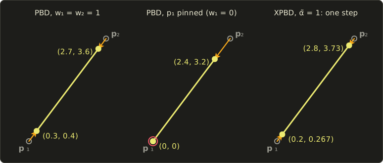
One constraint is solved exactly in one projection; a cloth has thousands that share particles, and fixing one breaks its neighbors, so PBD sweeps over all of them several times, exactly like the sequential impulses above (it's a nonlinear Gauss–Seidel iteration).
Stiffness depends on the iteration count
To make a constraint soft, PBD multiplies each correction by a stiffness .
But the correction is applied in every iteration, so after iterations the remaining error is : with that's 0.5 after one iteration, 0.0625 after 4, and 0.000015 after 16.
The same material gets stiffer when you raise the iteration count, and it also changes with the time step.
The PBD paper compensates with (for and , , and ), which fixes the iteration dependence but not the time-step dependence.
The cloth below shows the effect: the same simulation (a 1.2 m cloth of 13×13 particles hanging from two corners, structural and shear distance constraints with , three seconds at 60 Hz) with 1, 4 and 16 iterations per step.
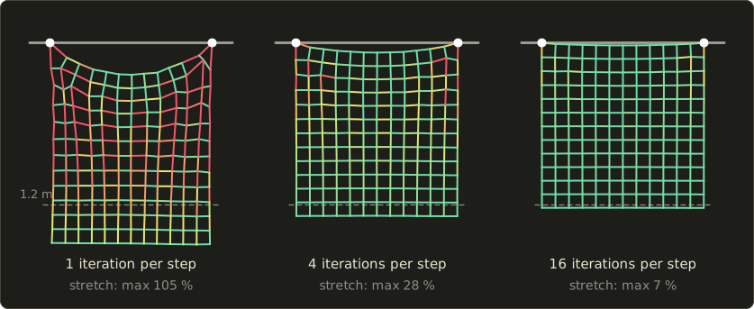
Even with "rigid" constraints, an iterative solver that stops early leaves the cloth stretchy, most of all near the pins, which carry the weight of everything below them.
Few iterations make rubber, many make cotton, and the result also depends on the resolution.
XPBD: compliance
XPBD (extended position-based dynamics; Macklin, Müller and Chentanez, Motion in Games 2016) fixes this by giving each constraint a physical compliance (コンプライアンス) , the inverse of its stiffness ( in m/N for a spring; 0 for a rigid rod), and by accumulating a Lagrange multiplier (ラグランジュ乗数) per constraint, which is the constraint's impulse.
With , each projection computes
and is reset to 0 at the start of each step.
With this is exactly the PBD projection.
Worked example.
The same two particles, now joined by a spring with N/m, so m/N; with s, .
First iteration: , so and .
The new length is , so .
Second iteration: : nothing changes, however many iterations follow.
The answer is a balance, not a projection: each particle was pulled m away from where inertia wanted it, which takes the force N, and the spring stretched by m pulls with N.
That's one implicit Euler step of the spring, solved by projection, and its result no longer depends on the iteration count: more iterations only bring a large system closer to the same answer.
Macklin and coworkers later showed ("Small Steps in Physics Simulation", SCA 2019) that many substeps with one iteration each beat few steps with many iterations at the same cost.
#include <cstdio>
#include "linalg.hh"

// XPBD distance constraint C = |p1 - p2| - d between two particles with inverse masses w1, w2.
// alpha is the compliance (1 / stiffness), h the time step, lambda the accumulated multiplier.
// With alpha = 0 this is exactly the PBD projection.
void solveDistance(Vec3 &p1, Vec3 &p2, float w1, float w2, float d, float alpha, float h,
                   float &lambda) {
  Vec3 delta = p1 - p2;
  float len = length(delta);
  if (len < 1e-9f || w1 + w2 == 0.0f) return;
  Vec3 n = delta / len;             // gradient of C with respect to p1
  float C = len - d;
  float alphaTilde = alpha / (h * h);
  float dLambda = (-C - alphaTilde * lambda) / (w1 + w2 + alphaTilde);
  lambda += dLambda;
  p1 = p1 + (w1 * dLambda) * n;
  p2 = p2 - (w2 * dLambda) * n;
}

int main() {
  const float alphas[] = {0.0f, 0.01f};  // rigid (PBD) and a spring of k = 100 N/m
  for (float alpha : alphas) {
    Vec3 p1{0, 0, 0}, p2{3, 4, 0};
    float lambda = 0.0f;
    for (int it = 1; it <= 2; ++it) {
      solveDistance(p1, p2, 1.0f, 1.0f, 4.0f, alpha, 0.1f, lambda);
      printf("alpha %.2f, iteration %d: p1 (%.4f, %.4f)  p2 (%.4f, %.4f)  "
             "length %.4f  lambda %.4f\n",
             alpha, it, p1.x, p1.y, p2.x, p2.y, length(p2 - p1), lambda);
    }
  }
  return 0;
}
With it prints the PBD result (length 4.0000, ), with the XPBD result (length 4.3333, ), and the second iteration changes nothing in either case.
Cloth with PBD
A PBD cloth uses the same particle grid as the mass–spring cloth of section 14.4, with constraints instead of springs:
- Stretch (伸び): distance constraints along the structural edges (and shear edges or a triangle area constraint against shearing).
- Bending (曲げ): either distance constraints that skip a particle, like bend springs, or a constraint on the dihedral angle (二面角) between neighboring triangles, which is independent of stretching.
- Collisions: inequality constraints that are projected only while violated, for example against a body surface or a signed distance field (chapter 21), and particle–triangle constraints for self-collision.
A Verlet cloth is the same thing written with Verlet integration: the velocity hides in , so relaxing the constraints by moving positions updates it by itself.
Long before PBD, Provot (Graphics Interface 1995) fixed stretchy mass–spring cloth with strain limiting (ひずみ制限): after each step, any spring stretched by more than a critical rate (10% for his hanging sheet) has its ends moved back to exactly that limit, both ends if both are free, only the free one if the other is pinned.
That's a PBD projection of the inequality , and cloth solvers still combine soft springs with such hard limits.
Shape matching
For soft objects that should spring back to a rest shape (jelly, cartoon squash and stretch), shape matching (シェイプマッチング; Müller, Heidelberger, Teschner and Gross, "Meshless Deformations Based on Shape Matching", SIGGRAPH 2005) needs no mesh at all.
Each step it finds the rigid motion (rotation and translation) that best matches the rest positions to the current positions , and pulls every particle a fraction of the way towards its goal position :
where is the rest center of mass and the rotation part of (its polar decomposition (極分解) ).
In 2D the rotation angle is simply .
Worked example.
A square of four unit masses rests at , so .
It has rotated by 90° and been dented: .
The center is , and the offsets are , , , .
Summing the outer products with the :
so : the dent didn't fool it.
The goals are the rest square rotated by 90° and moved to : , , , .
With , the dented corner moves from halfway to its goal, to .
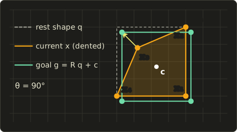
Matching with the full matrix instead of allows stretching modes, and overlapping clusters give local wobble.
The finite element method, briefly
Mass–spring systems and PBD are fast, but their stiffness depends on the mesh, and it's hard to say "this is rubber".
The finite element method (有限要素法, FEM) starts from continuum mechanics instead.
The material is split into tetrahedra (in 2D, triangles), and inside each element the deformation is assumed to be linear, described by the deformation gradient (変形勾配)
where the columns of are the element's edge vectors at rest and those of the same edges now.
Strain (ひずみ) measures the deformation, stress (応力) the internal force per area, and linear elasticity connects them with Hooke's law in matrix form, using Young's modulus (ヤング率; roughly 0.01 to 0.1 GPa for rubber, 200 GPa for steel) and Poisson's ratio (ポアソン比; how much the material thins when stretched, near 0.5 for rubber).
Worked example.
A 2D triangle with rest corners , , has .
Stretched to in x, and the linear strain .
Now only rotate it by 90°, to , , : and , a 100% compression for a triangle that isn't deformed at all.
Linear FEM therefore produces ghost forces for spinning objects.
Corotational FEM (共回転FEM) removes the rotation first with the polar decomposition of shape matching (, strain from ); nonlinear models use the Green strain , which is 0 for any rotation.
The element forces assemble into the sparse stiffness matrix of section 26.1 and are integrated implicitly; film uses FEM for muscles and flesh, and at the time of writing PhysX offers GPU FEM soft bodies.
26.4 Fluids in depth
The Navier–Stokes equations, term by term
For a fluid with velocity field , pressure , constant density and kinematic viscosity , the incompressible Navier–Stokes equations (ナビエ・ストークス方程式) of section 14.7 read
("nabla") is the vector of partial derivatives , and each term is one physical effect:
- , advection (移流): the fluid carries its own velocity along. It's the reason for swirls and the hard, nonlinear part.
- , pressure (圧力): fluid is pushed from high to low pressure. Pressure is whatever it must be to keep the fluid incompressible.
- , viscosity (粘性): velocity diffuses to the neighbors; (the Laplacian, ラプラシアン) is "the average of the neighbors minus me". Honey has a large , air a tiny one.
- : external forces such as gravity, buoyancy or a stirring hand.
- : the divergence (発散), the net outflow per volume, is zero. What flows into a cell must flow out: incompressibility (非圧縮性).
Every quantity the fluid carries (smoke density, temperature, dye) follows the advection part alone: .
Stable Fluids
Jos Stam's Stable Fluids (SIGGRAPH 1999), named in section 14.7, solves these equations on a grid by operator splitting (演算子分割): one step applies the terms one after another, each with a method that is stable for any time step.
- Add forces: .
- Advect with the semi-Lagrangian method (セミラグランジュ法): to find the new value at a grid point, trace backwards along the velocity to where the fluid came from, , and interpolate the old field there.
- Diffuse implicitly: solve (implicit Euler again, so any and are fine). Smoke and water often skip this step, because the numerical diffusion of step 2 is already more than enough.
- Project: remove the divergence by solving a Poisson equation (ポアソン方程式) for the pressure and subtracting its gradient. This uses the Helmholtz–Hodge decomposition (ヘルムホルツ・ホッジ分解): any vector field is a divergence-free part plus a gradient, and the projection keeps only the first.
Worked example: semi-Lagrangian advection.
A 1D row of cells with spacing 1 holds the smoke density at , and the velocity is everywhere, with .
For the cell at , the fluid came from , between and : .
At : from 2.4, ; at : from 1.4, .
The new row is : the block moved 0.6 cells to the right, its total is still 2, and its edges got blurred.
With a much larger step, , on a longer row , the result is : still sensible.
Every new value is an interpolation of old values, so it can never leave the old range: that's why this step can't blow up.
A naive explicit difference scheme ("upwind", ) gives the same at , but at it produces : negative smoke and a growing spike.
Explicit schemes need , the CFL condition (CFL条件, after Courant, Friedrichs and Lewy).
The price of the semi-Lagrangian step is numerical dissipation (数値散逸): the blurring repeats every step, swirls fade, and smoke looks thick and syrupy.
On the GPU, advection is one texture lookup per cell, the bilinear interpolation done by the sampler (you'll meet compute shaders in the GLSL series, chapter 15):
Texture2D<float2> velocity;
Texture2D<float4> source;
SamplerState linearClamp;

// Semi-Lagrangian advection: fetch the value from where the fluid came from.
// uv: this cell's texture coordinate, h: time step, u is stored in cells per second.
float4 advect(float2 uv, float h, float2 invGridSize) {
  float2 u = velocity.SampleLevel(linearClamp, uv, 0);
  float2 back = uv - h * u * invGridSize;
  return source.SampleLevel(linearClamp, back, 0);
}layout(set = 0, binding = 0) uniform sampler2D velocity;
layout(set = 0, binding = 1) uniform sampler2D source;
// Semi-Lagrangian advection: fetch the value from where the fluid came from.
// uv: this cell's texture coordinate, h: time step, u is stored in cells per second.
vec4 advect(vec2 uv, float h, vec2 invGridSize) {
vec2 u = textureLod(velocity, uv, 0.0).xy;
vec2 back = uv - h * u * invGridSize;
return textureLod(source, back, 0.0);
}Texture2D<float2> velocity;
Texture2D<float4> source;
SamplerState linearClamp;
// Semi-Lagrangian advection: fetch the value from where the fluid came from.
// uv: this cell's texture coordinate, h: time step, u is stored in cells per second.
float4 advect(float2 uv, float h, float2 invGridSize) {
float2 u = velocity.SampleLevel(linearClamp, uv, 0);
float2 back = uv - h * u * invGridSize;
return source.SampleLevel(linearClamp, back, 0);
}Pressure projection on a 2×2 grid
Grid solvers usually store velocities on the cell faces and pressure at the cell centers, the MAC grid (MAC格子, a staggered grid, スタッガード格子), because the divergence of a cell and the pressure difference across a face then fall out naturally.
With grid spacing 1, and :
- The divergence of a cell is (right face u − left face u) + (top face v − bottom face v).
- The projection subtracts the pressure difference across each face: , and the same for v with top and bottom.
- For the result to have zero divergence, the pressure must satisfy, in every cell, . Wall faces have velocity 0 and add no term.
Worked example.
Four cells in a box with solid walls; only the face between the two bottom cells has a velocity, (fluid pushed to the right).
The bottom-left cell loses fluid (divergence +1), the bottom-right one gains it (−1), the top cells are 0.
Each cell has two fluid neighbors, so the update for one cell is .
One Gauss–Seidel sweep, starting from all zeros, in the order bottom-left, bottom-right, top-left, top-right:
A second sweep changes nothing, so this tiny system is solved (pressure is only defined up to a constant; only differences matter).
The new face velocities: bottom , top , left column , right column .
Check the bottom-left cell: out through the right face 0.25, out through the top face −0.25 (that's inflow): divergence 0, and the other three cells balance the same way.
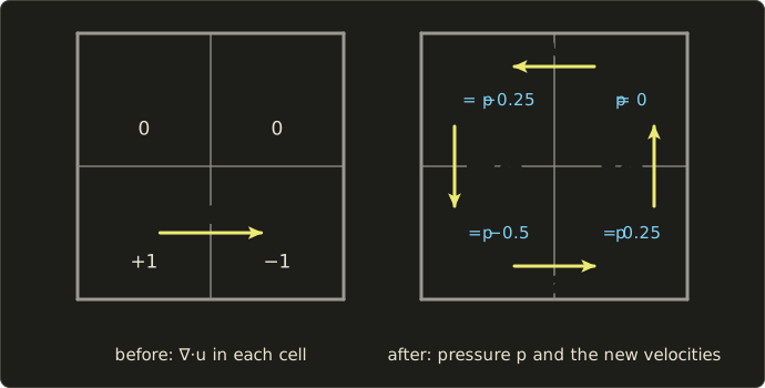
The push to the right became a small counter-clockwise vortex: in a closed box the fluid has nowhere to go but around.
Only a quarter of the original speed survives, because the projection keeps the divergence-free part and throws the rest away.
Real grids have to cells, and the Poisson solve (preconditioned conjugate gradients, multigrid, or on the GPU a fixed number of Jacobi iterations) dominates the cost.
On this particular grid plain Jacobi (all cells updated from the old values at once) actually oscillates between two states forever; weighted Jacobi, which moves only two thirds of the way each time, converges (the bottom face goes 0.333, 0.333, 0.259, 0.259, 0.251, … towards 0.25).
Smoke and fire
Smoke adds two fields that are advected with the flow, the smoke density and the temperature , and a buoyancy (浮力) force (Fedkiw, Stam and Jensen, "Visual Simulation of Smoke", SIGGRAPH 2001):
Heavy smoke sinks, hot gas rises.
The same paper introduced vorticity confinement (渦度閉じ込め): measure the swirl (the vorticity, the curl of ), and add a force that spins the small vortices back up, to give back the detail that numerical dissipation removes.
Fire adds a fuel or reaction field, expansion where fuel burns, and a color from the temperature (the blackbody colors of chapter 3).
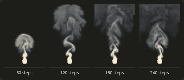
The run above is a toy version (72×112 cells, semi-Lagrangian advection, buoyancy, a little vorticity confinement, 60 Jacobi iterations per step) that shows the density as brightness; rendering smoke with light scattering inside it is volume rendering, chapter 28.
SPH: kernels and density
In SPH (section 14.7) every quantity at a point is a weighted sum over nearby particles, with a smoothing kernel (平滑化カーネル) that is largest at distance 0 and falls to 0 at the support radius (here is a radius, not the time step).
Müller, Charypar and Gross (2003) chose a different kernel for each job:
Both integrate to 1 over the ball of radius .
Poly6 is used for density, because it only needs (no square root).
But its slope is 0 at the center, so two particles very close together feel no pressure force and clump; the pressure force therefore uses the spiky kernel, whose slope is largest at the center.
(A third kernel with a positive Laplacian is used for viscosity.)
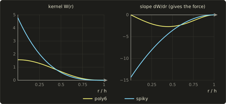
Worked example: density.
With (in units of the kernel radius), , and .
A particle has neighbors at distances 0.5, 0.5 and 0.8; all masses are 1.
It counts itself too ():
The equation of state (状態方程式) turns density into pressure: with and a rest density , , so this crowded particle pushes its neighbors away.
The pressure force is , symmetric so that two particles push each other equally.
This "weakly compressible" SPH needs a large to keep water from compressing, which makes it stiff.
Later methods enforce incompressibility with a solver (PCISPH, IISPH, DFSPH), and position-based fluids (Macklin and Müller, SIGGRAPH 2013) make a PBD constraint per particle, as PhysX's GPU fluids do at the time of writing.
Neighbors are found with a uniform grid of cell size .
PIC, FLIP and APIC
Grids are good at pressure and bad at advection; particles are the opposite, so hybrid methods (ハイブリッド法) use both every step:
- P2G: transfer the particle velocities to the grid (a kernel-weighted average onto the nearby faces).
- Solve forces and the pressure projection on the grid.
- G2P: transfer the velocities back, then move the particles through the grid velocity field.
The question is how to transfer back.
PIC (particle-in-cell) gives each particle the interpolated new grid velocity, which averages away everything finer than the grid: smooth, stable and very dissipative.
FLIP (fluid-implicit-particle; Brackbill and Ruppel, 1986) adds only the change of the grid velocity to the particle's own velocity, which keeps the particle's detail but also its noise.
Zhu and Bridson ("Animating Sand as a Fluid", SIGGRAPH 2005) adapted both to incompressible flow and brought them into graphics, suggesting a weighted average to tune the numerical viscosity (PIC for sand, FLIP for water).
Worked example.
A particle carries 2.4 m/s.
At its position, the grid velocity was 2.0 m/s after P2G and is 1.5 m/s after the pressure solve.
PIC: the particle gets 1.5.
FLIP: .
A blend of, for example, 95% FLIP and 5% PIC: .
APIC (the affine particle-in-cell method; Jiang, Schroeder, Selle, Teran and Stomakhin, SIGGRAPH 2015) gives each particle a small matrix describing how the velocity varies around it (a locally affine velocity), and transfers it both ways.
This keeps rotation, conserves angular momentum exactly across the transfers, and removes PIC's dissipation without FLIP's noise.
MPM (the material point method, 物質点法), from computational mechanics in the 1990s, takes the hybrid idea to solids.
Particles carry mass, velocity and a deformation gradient like the FEM of section 26.3; the grid computes the stress forces each step; nothing ever has to be meshed or remeshed, so the material can tear, flow, merge and pile up.
Stomakhin, Schroeder, Chai, Teran and Selle ("A Material Point Method for Snow Simulation", SIGGRAPH 2013) used it for the snow of Disney's Frozen, and MPM is now used for sand, mud, foam and other materials that are half solid and half fluid.
Rendering water
The simulation only gives particles or a grid; the picture needs a surface and a material:
- Surface: an implicit function built from the particles, polygonized with marching cubes (chapter 9, section 9.3), or a level set (a signed distance field, chapter 21) on the grid; games often splat particles into a depth buffer and shade it in screen space.
- Shading: Fresnel reflection (chapter 22), refraction, absorption that tints deep water (chapter 28), caustics, and spray, foam and bubbles as extra particles.
- Oceans are usually not simulated: a sum of many waves with a measured spectrum, computed with an FFT, gives a tileable height field.
26.5 Hair, destruction and simulation in practice
Hair
Section 14.4 described a strand as a chain of particles with stretch and bend springs, with guide hairs and interpolation for the rest.
Hair is almost inextensible, the worst case for stiff springs, and it twists.
Two directions dominate:
- Position-based chains. "Follow the leader" (Müller, Kim and Chentanez, VRIPHYS 2012) projects each particle to the right distance from its predecessor in one pass from root to tip, so the strand is exactly inextensible, and corrects the velocities to hide the resulting bias.
- Rods. Film hair uses elastic rod models that include twist, solved implicitly.
Destruction with Voronoi fracture
Section 14.7 described destruction as pre-fractured pieces glued with breakable constraints.
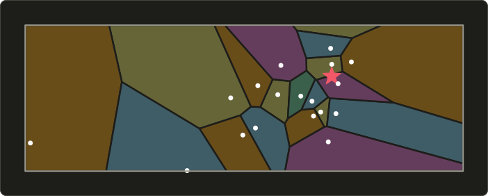
The pieces usually come from a Voronoi diagram (ボロノイ図): scatter seed points (more near the expected impact point, for small splinters there and large chunks far away), and give every point of the object to the nearest seed.
Each Voronoi cell is the intersection of half-spaces, one per other seed, bounded by the perpendicular bisector (垂直二等分線) of the two seeds, so every piece is convex: perfect for convex collision shapes and GJK.
Worked example.
Seeds and .
A point is equally far from both when , which simplifies to , or .
The point has , so it belongs to (check: squared distances 2 and ).
To cut a cell, clip the object's polygon (or mesh) against each bisector with exactly the half-plane clipping of chapter 6.
Physics on the GPU
GPUs need thousands of independent tasks (chapter 29).
Particles, grid fluids (advection is one lookup per cell, Jacobi is one stencil per cell), SPH and PBD map well; rigid bodies with their branchy narrow phase and sequential constraint solving are harder.
The Gauss–Seidel solvers of this chapter are sequential by nature (each constraint uses its neighbors' newest values), and the GPU uses two answers:
- Jacobi (ヤコビ法): every constraint computes its correction from the old positions, and the corrections are averaged per particle. Fully parallel, but slower to converge.
- Graph coloring (グラフ彩色): split the constraints into groups (colors) in which no two share a particle, run each group in parallel and the groups in sequence: still exact Gauss–Seidel. The cloth of section 26.3 used 8 colors (horizontal, vertical, diagonal and anti-diagonal constraints, each split in two by the parity of the column, or of the row for the vertical ones).
At the time of writing, engines such as NVIDIA PhysX run rigid bodies, PBD particles (fluids, granular material) and FEM soft bodies on CUDA GPUs, and many games run cloth, hair and particle effects in compute shaders.
Determinism and networking
A simulation is deterministic (決定的) when the same inputs give bit-for-bit the same result.
That sounds automatic, but floating-point arithmetic isn't associative.
In single precision, but , because rounds back to .
A different summation order (thread schedule, SIMD width), a compiler that fuses a multiply and an add into one FMA instruction, or a different sin can change the last bit, and chaotic systems (a falling stack, a breaking wall) amplify that into different outcomes within seconds.
Determinism on one machine needs a fixed time step (section 14.8), a fixed order of bodies and contacts (sort them, don't rely on hash-table order) and no uninitialized data.
Determinism across platforms also needs control of the compiler's floating-point settings; at the time of writing, Jolt Physics, for example, has a build option that aims to give the same results on all platforms.
Multiplayer games choose between two strategies:
- Lockstep (ロックステップ): every machine runs the full simulation and only the inputs are sent. Little bandwidth (popular in strategy games with thousands of units), but it needs perfect determinism.
- State synchronization (状態同期): a server runs the authoritative simulation and sends object states. Clients predict their own player (client-side prediction, クライアント側予測) and, when the server disagrees, rewind and replay their inputs (rollback, ロールバック). More bandwidth, but small differences don't matter.
Exam points
These tie back to the syllabus item physics-based animation (chapter 14) and are worth being sure about for the exam:
- Explicit Euler uses the current state and is unstable for an undamped spring at every step size; implicit (backward) Euler uses the end of the step, needs equation solving, is stable for any step and damps artificially; semi-implicit Euler is stable while .
- Collision detection is broad phase then narrow phase; two convex shapes are separate exactly when some axis separates their projections (SAT); the response is an impulse along the contact normal, with friction limited by times the normal impulse.
- Mass–spring cloth with stiff springs needs small steps or implicit integration; position-based methods move positions to satisfy constraints directly.
- Fluids: Eulerian grids (Stable Fluids: advection, diffusion, pressure projection) vs Lagrangian particles (SPH), and hybrids that use both.
26.6 Summary
- Implicit Euler divides a spring's energy by per step: stable for any step (A-stable), but damped; explicit Euler's stability region misses the imaginary axis.
- Rigid bodies need the world inertia tensor , a normalized quaternion update and care with the gyroscopic term.
- SAT gives separation, normal and depth (4 axes for 2D boxes, 15 for 3D); clipping builds the contact manifold; GJK and EPA work for any convex shape through support functions.
- Sequential impulses (projected Gauss–Seidel) clamp accumulated impulses (, ) and rely on warm starting, Baumgarte bias with slop, and sleeping; joints and motors are solved in the same sweeps.
- PBD projects positions onto constraints; XPBD's compliance makes stiffness independent of the iteration count. Strain limiting, shape matching and corotational FEM build on the same ideas.
- Stable Fluids: forces, semi-Lagrangian advection, implicit diffusion, pressure projection. SPH: poly6 for density, spiky for pressure. PIC, FLIP and APIC transfer velocities between particles and grid; MPM handles snow and sand.
- Hair uses inextensible chains or rods, destruction convex Voronoi pieces, GPUs Jacobi or graph coloring; determinism needs a fixed step, a fixed order and controlled floating point.
26.7 Key terms
| English | 日本語 |
|---|---|
| stiff system | 硬い系(スティッフな系) |
| implicit (backward) Euler method | 陰的オイラー法(後退オイラー法) |
| stability region | 安定領域 |
| A-stable | A安定 |
| stiffness matrix | 剛性行列 |
| conjugate gradient method | 共役勾配法 |
| angular momentum | 角運動量 |
| principal axes of inertia | 慣性主軸 |
| gyroscopic term | ジャイロ項 |
| separating axis theorem (SAT) | 分離軸定理(SAT) |
| contact manifold | 接触点の集合(コンタクトマニフォールド) |
| reference face, incident face | 参照面、入射面 |
| support function | サポート関数 |
| Minkowski difference | ミンコフスキー差 |
| GJK, EPA | GJK法、EPA |
| effective mass | 有効質量 |
| Coulomb friction, friction cone | クーロン摩擦、摩擦円錐 |
| sequential impulses | シーケンシャルインパルス |
| projected Gauss–Seidel (PGS) | 射影ガウス=ザイデル法(PGS) |
| joint, motor | ジョイント、モーター |
| Baumgarte stabilization, slop | バウムガルテ安定化、許容めり込み(スロップ) |
| warm starting | ウォームスタート |
| sleeping, island | スリープ、アイランド |
| position-based dynamics (PBD) | 位置ベース動力学(PBD) |
| compliance (XPBD) | コンプライアンス(XPBD) |
| strain limiting | ひずみ制限 |
| shape matching | シェイプマッチング |
| polar decomposition | 極分解 |
| finite element method (FEM) | 有限要素法(FEM) |
| deformation gradient | 変形勾配 |
| strain, stress | ひずみ、応力 |
| Young's modulus, Poisson's ratio | ヤング率、ポアソン比 |
| corotational FEM | 共回転FEM |
| advection | 移流 |
| divergence, incompressibility | 発散、非圧縮性 |
| semi-Lagrangian method | セミラグランジュ法 |
| pressure projection | 圧力投影 |
| Poisson equation | ポアソン方程式 |
| Helmholtz–Hodge decomposition | ヘルムホルツ・ホッジ分解 |
| MAC grid (staggered grid) | MAC格子(スタッガード格子) |
| CFL condition | CFL条件 |
| numerical dissipation | 数値散逸 |
| buoyancy | 浮力 |
| vorticity confinement | 渦度閉じ込め |
| smoothing kernel | 平滑化カーネル |
| PIC, FLIP, APIC | PIC法、FLIP法、APIC法 |
| material point method (MPM) | 物質点法(MPM) |
| Voronoi diagram | ボロノイ図 |
| Jacobi method, graph coloring | ヤコビ法、グラフ彩色 |
| determinism | 決定性 |
| lockstep, state synchronization | ロックステップ、状態同期 |
| client-side prediction, rollback | クライアント側予測、ロールバック |
26.8 Challenges
- ★ A mass kg hangs on a spring with N/m, m, . Compute two steps of implicit Euler with s and the energy after each. By what factor does each step change the energy, and what would explicit Euler's factor be?
- ★ A box of 6 kg has the sides 1, 2 and 3 m along its local x, y and z axes. Compute , then after a rotation by 90° about z, and the angular velocity for . Is it parallel to ?
- ★★ Box A is axis-aligned at the origin with half-extents ; box B has half-extents , axes , and its center at . Run SAT on all four axes, give the contact normal and the depth, then move B to and say which axis separates them.
- ★★ A rope of three particles hangs straight down: pinned, , , all other , rest lengths 1. Do two PBD sweeps (constraint 1–2, then 2–3) and give the lengths after each. Then do one sweep with XPBD and for both constraints. Which one is closer to the rest lengths, and why is that not a flaw?
- ★★ In the 2×2 box of section 26.4, start instead with only the face between the two top cells moving, (to the left). Compute the divergences, one Gauss–Seidel sweep for the pressure (same order), and the four new face velocities. Check that every cell has zero divergence, and say which way the vortex turns.
- ★★★ A tower of ten boxes jitters and slowly sinks into the ground. Explain the role of solver iterations, warm starting, the Baumgarte factor and slop, the contact order and sleeping, which you'd change first, and the side effects you'd expect.
Multiple choice
Q1 ★ Which of the following statements about integrating a stiff spring is correct?
| A | Implicit Euler stays stable for an undamped spring at any time step, but it removes energy every step, so the oscillation dies out faster than it should. |
| B | Explicit Euler is stable for an undamped spring as long as . |
| C | Implicit Euler needs no equation solving, so it costs the same as explicit Euler for a cloth with thousands of springs. |
| D | The stability region of explicit Euler contains the whole left half of the complex plane. |
| E | The stiffer the spring, the larger the time step that explicit methods can use. |
Q2 ★★ Which of the following statements about rigid-body contact is correct?
| A | For two boxes in 3D, SAT only has to test the six face normals of the two boxes. |
| B | In sequential impulses, the accumulated normal impulse of each contact is clamped to be non-negative, and the friction impulse is clamped to at most times the normal impulse in size. |
| C | GJK is a broad-phase method that sorts the bounding boxes of all bodies along one axis. |
| D | Warm starting means running more solver iterations in the first frame of a simulation. |
| E | The inertia tensor in world space is the same for every orientation of a body, so it is computed once. |
Q3 ★★ Which of the following statements about simulation methods is correct?
| A | Semi-Lagrangian advection traces particles forward in time and is stable only when the CFL number is below 1. |
| B | The pressure projection of Stable Fluids adds divergence to the velocity field so that the fluid can expand. |
| C | FLIP transfers only the change of the grid velocity back to the particles, which keeps detail but adds noise, while PIC copies the grid velocity, which is smooth but dissipative. |
| D | In XPBD, the stiffness of a constraint depends more strongly on the iteration count than in PBD. |
| E | SPH computes the density of a particle by solving a Poisson equation on a grid. |
26.9 Practical assignment
A crate, a rope and a puff of smoke, by hand.
You need graph paper, a pencil, a ruler and a calculator; you'll take one step of each kind of solver in this chapter.
- Explicit vs implicit. A spring with N/m and kg starts at m, . Take one step with s with explicit Euler and one with implicit Euler (use the closed form of section 26.1), and compute the energy before and after each.
- SAT. On graph paper, draw box A (center , axis-aligned, half-extents ) and box B (center , half-extents , axes , ). Compute the overlap on all four axes, choose the contact normal and depth, and draw the normal on your sketch.
- Impulse with friction. Repeat the crate of section 26.2 (, , , , ) with . Do two sequential-impulse iterations by hand (normal, then friction, clamping the accumulated values), then solve the sliding case exactly as in the text.
- PBD rope. Three particles hang at (pinned), and , at rest, with rest lengths 1. With m/s² and s, predict the positions, do two sweeps of distance projections (1–2, then 2–3), and compute the new velocities from the position change.
- Pressure projection. In the 2×2 box of section 26.4, the face between the two left cells has (up), all others 0. Compute the divergences, one Gauss–Seidel sweep for the pressure, and the new face velocities. Draw the result as arrows.
- SPH density. With and unit masses, compute the poly6 density at for particles at , , and .
How to check yourself:
- Step 1: the energy starts at 2 J; explicit Euler doubles it and implicit Euler halves it (), and the implicit result satisfies .
- Step 2: all four overlaps are positive; the smallest is on A's y axis, so the normal is and the depth is less than 0.5.
- Step 3: after iteration 1 the friction impulse sits at its limit , the remaining shrinks each iteration, and the exact lies between 0.8 and 1 with the contact still sliding.
- Step 4: after each sweep the second length is exactly 1 and the first is slightly too long, half as much after the second sweep; both moving particles get the same small downward velocity.
- Step 5: every face has speed 0.25, all four cells have zero divergence, and the arrows form a loop (it turns clockwise this time).
- Step 6: the particle at is exactly at distance and contributes nothing; the density is a little below 2.9.
コメント(0)
まだコメントはありません。
ログインするとコメント出来ます。