11. Shadows and Mapping
In chapter 10 we decided which surface is visible in each pixel and how bright it is under a light.
Two things are still missing, and without them every CG image looks fake.
The first is shadows: a lit surface is only lit if nothing stands between it and the light.
The second is detail: real surfaces have wood grain, scratches, bricks and dents, and modeling every one of them as polygons would be impossible.
In this chapter we add both: first the classic shadow algorithms, then texture mapping and its many relatives (bump, normal, displacement, environment and procedural maps).
Why does this matter?
Shadows and textures are two of the depth cues from chapter 3 (section 3.9), so they decide whether a picture reads as 3D at all.
And in a real-time renderer, most of the frame's memory and a large part of its time go into exactly these two things: shadow maps and textures.
For the exam, this chapter covers two syllabus items of area 4, shadowing (影付け) and mapping (マッピング).
It builds on the projection matrices of chapter 5, the pipeline and rasterization of chapter 6, and sampling and aliasing from chapter 2.
11.1 Shadows: what they are and why they matter
Look at a ball on a table.
Two different dark areas appear:
- the side of the ball that faces away from the lamp is dark because the light hits it at a grazing angle or not at all: that's the attached shadow or shade (陰, in);
- the dark patch on the table is dark because the ball blocks the light: that's the cast shadow (影, kage).
Japanese keeps the two apart with two different characters, which is worth remembering for the exam.
The first one is already handled by shading: when the angle between the normal and the light direction is more than 90°, the diffuse term of chapter 10 drops to zero.
The second one needs to know about other objects, and that's what this chapter adds.
When an object casts a shadow onto itself (an arm onto the body, the nose onto a cheek), we call it self-shadowing (セルフシャドウ).
Cast shadows do a lot of work for the viewer:
- Position and contact. Without a shadow, you can't tell whether a ball lies on the floor or floats above it. The shadow "glues" objects to the ground.
- Shape. A shadow falling over a bumpy surface shows the bumps.
- Light direction. Shadows tell you where the light is, which makes the whole scene consistent.
Umbra and penumbra
A point light (点光源) is a single point, so every point of the scene either sees it or doesn't.
The shadow has a sharp edge: a hard shadow (ハードシャドウ).
A real lamp, a window or the sky is an area light (面光源) with a size.
A point on the floor can then see all of it, none of it, or part of it:
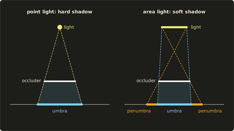
- the umbra (本影, hon'ei) is the part where the whole light is hidden: fully dark;
- the penumbra (半影, han'ei) is the part where only some of the light is hidden: a gradient from dark to lit.
A shadow with a penumbra is a soft shadow (ソフトシャドウ).
How wide is the penumbra?
Take a light of width at height above the floor and an occluder edge at height .
The two rays from the two ends of the light through the occluder edge form two similar triangles, and the width of the penumbra on the floor is
Worked example. A ceiling light 1 m wide at a height of 4 m and the edge of a table at 1 m:
A box lying on the floor has its edge at only 0.1 m, so its shadow's penumbra is m, about 2.6 cm.
That's why shadows are sharp near the point of contact and get softer the farther they are from the occluder (contact hardening), and why a renderer that blurs every shadow by the same amount looks wrong.
In the figure the light is 1.6 wide at height 5 and the occluder at 1.5, so the penumbra is wide on each side.
Shadows are hidden surfaces seen from the light
Here is the key idea behind every shadow algorithm:
A point is in shadow exactly when it is hidden from the light.
So shadowing is hidden surface removal again (chapter 10), done once more with the eye replaced by the light.
The algorithms below differ in how they do that second visibility test: by projecting geometry (11.2), by building volumes (11.3), with a depth image (11.4) or by tracing rays (11.5).
11.2 Projected shadows onto a plane
The oldest and simplest trick, the projected shadow or planar shadow method (投影法), works when shadows only fall onto one flat plane, like the floor.
Each vertex of the object is projected along the ray from the light onto the plane, and the projected object is drawn in a dark color.
That projection is a perspective projection with the light as the center of projection (chapter 5), so it can be written as one 4×4 matrix.
The shadow matrix for the plane y = 0
Take the light at and a point below it ().
The ray reaches at , which gives the shadow point
The common denominator is exactly what homogeneous coordinates handle (Linear Algebra chapter 9): put the numerators in x, y, z, the denominator in w, and let the division by w do the rest.
For any plane (the points with ) and the light in homogeneous form, the same matrix is
where is a 4×1 column times a 1×4 row, a 4×4 matrix (Linear Algebra chapter 7).
It's easy to see why it works.
is a combination of and , so it lies on the line through the light and the point.
And , so it lies on the plane.
With you get the matrix above.
For a directional light (平行光源) like the sun, use , the direction towards the light: then w stays for every point, the matrix is affine, and the formula becomes , a parallel projection.
A worked example
Light at , a box from to on the floor.
Here , so
The top corner :
Check with the ray: , and .
The other top corner on the light's side, , lands at , under the box itself, and the bottom corners stay where they are, because makes .
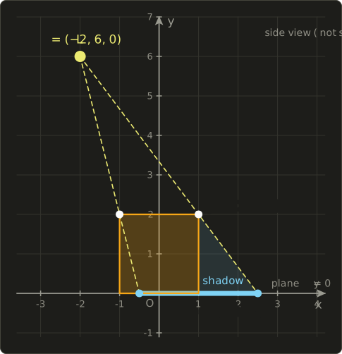
The same matrix in C++ with linalg.hh, as a check of the hand calculation:
#include <cstdio>
#include "linalg.hh"

// Shadow projection onto the plane a x + b y + c z + d = 0 from the light l
// (l.w = 1: point light at l.xyz, l.w = 0: directional light towards l.xyz).
// M = (plane . l) I - l plane^T
Mat4 shadowMatrix(Vec4 plane, Vec4 l) {
  float pl[4] = {plane.x, plane.y, plane.z, plane.w};
  float lv[4] = {l.x, l.y, l.z, l.w};
  float d = dot(plane, l);
  Mat4 m;
  for (int row = 0; row < 4; ++row) {
    for (int col = 0; col < 4; ++col) {
      m.at(row, col) = (row == col ? d : 0.0f) - lv[row] * pl[col];
    }
  }
  return m;
}

int main() {
  Mat4 s = shadowMatrix({0, 1, 0, 0}, {-2, 6, 0, 1}); // ground y = 0, light at (-2, 6, 0)
  for (int row = 0; row < 4; ++row) {
    printf("%4g %4g %4g %4g\n", s.at(row, 0), s.at(row, 1), s.at(row, 2), s.at(row, 3));
  }
  Vec4 p{1, 2, 1, 1};
  Vec4 q = s * p;
  printf("homogeneous (%g, %g, %g, %g)\n", q.x, q.y, q.z, q.w);
  printf("shadow point (%g, %g, %g)\n", q.x / q.w, q.y / q.w, q.z / q.w);
  return 0;
}
   6    2    0    0
   0    0    0    0
   0    0    6    0
   0   -1    0    6
homogeneous (10, 0, 6, 4)
shadow point (2.5, 0, 1.5)
In practice and limits
To draw the shadow, render the object a second time with the shadow matrix inserted between its model matrix and the view matrix, , in a dark color and without lighting.
Three practical problems come up at once:
- The flattened object lies exactly in the floor plane, so the two fight in the depth buffer (z-fighting, section 10.3). The usual cure is a small depth offset, or drawing the shadow with the stencil test.
- Overlapping triangles of the flattened object would darken the floor twice when the shadow is drawn semi-transparent. The stencil buffer (chapter 6) can mark each floor pixel so it is darkened only once.
- A point above the light () gets a negative w and projects to the wrong side: a false "anti-shadow". Such points must be clipped away.
And the big limitation: the shadow only falls on that one plane.
No shadows on curved surfaces, on other objects or on the object itself.
It was popular in early 3D games for characters on a flat floor, and an even cheaper cousin, a dark blurred disc under each character (a blob shadow), is still common today.
11.3 Shadow volumes
The shadow volume method (シャドウボリューム法) was proposed by Frank Crow in 1977.
It describes the shadowed region of space as geometry.
The idea
Find the silhouette edges (シルエットエッジ) of the occluder as seen from the light: the edges shared by one triangle facing the light and one facing away from it.
Extrude each silhouette edge away from the light (to infinity, or far enough) to a quadrilateral.
Together with the occluder itself, these quads close off a region of space behind it: the shadow volume.
Every point inside the volume is in shadow, every point outside is lit (by this light, as far as this occluder is concerned).
Counting with the stencil buffer
How do we know whether the visible point of a pixel lies inside a volume?
Walk along the ray from the eye to that point and count the volume's faces it crosses: entering through a face turned towards the eye (a front face) adds 1, leaving through a face turned away (a back face) subtracts 1.
If the count is not zero, the point is inside a volume, so it is in shadow.
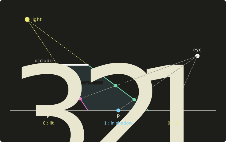
In the picture the volume has two side faces: the green one faces the eye (+1) and the pink one faces away (−1).
- : the eye ray crosses no face, count 0, lit.
- : the eye ray enters through the green face and stops inside, count 1, in shadow.
- : the eye ray enters (+1) and leaves (−1) before reaching the ground, count 0, lit. The point is behind the shadow volume, not inside it.
Tim Heidmann showed in 1991 how a GPU can do this count with the stencil buffer (ステンシルバッファ), a small integer per pixel (chapter 6):
- Draw the whole scene with ambient light only, which also fills the depth buffer.
- With depth writes and color writes off, draw the front faces of all shadow volumes and add 1 to the stencil value wherever the depth test passes (the face is in front of the visible surface).
- Draw the back faces and subtract 1 wherever the depth test passes.
- Draw the scene again with the light switched on, but only where the stencil value is 0.
Faces in front of the visible point pass the depth test, so steps 2 and 3 count exactly the crossings between the eye and that point.
This is called depth pass or z-pass (Zパス法).
Several overlapping volumes simply add up, which is why the test is "not zero" and not "equals one".
Z-pass and z-fail
Z-pass has one weak spot: if the eye itself is inside a shadow volume (the camera stands in the shadow of a pillar), the ray starts inside without crossing an entering face, all counts are off by one, and lit and shadowed areas swap.
The fix counts the other half of the ray instead, from the visible point to infinity: add 1 for back faces that fail the depth test (they lie behind the visible point) and subtract 1 for front faces that fail.
For above, the part of the ray behind the point leaves the volume once through a back face, +1, in shadow again; for nothing lies behind it, 0, lit.
This depth fail or z-fail method (Zフェイル法) was found by Bilodeau and Songy (1998) and independently by John Carmack (2000), so it's also called "Carmack's reverse"; the volumes must then be closed at both ends with caps.
Doom 3 (2004) is the famous game that lit its whole world with stencil shadow volumes.
Strengths and weaknesses
- Pixel-exact hard shadows on every surface, including self-shadowing, with no resolution problems.
- But: silhouette edges must be found on the CPU or in a geometry stage, meshes must be closed (2-manifold, chapter 7), and the huge extruded quads cost a lot of fill rate.
- Only hard shadows. Soft shadows need many volumes from many light positions.
Because of the fill-rate cost and the lack of soft edges, most modern engines use shadow maps instead.
11.4 Shadow mapping
Shadow mapping (シャドウマッピング) was introduced by Lance Williams in 1978.
It does the visibility test from the light with a depth buffer, which a GPU is very good at.
Two passes
- Render from the light. Put a camera at the light, looking where the light shines, and render only depths. The result is the shadow map (シャドウマップ, also depth map): for each texel, the distance to the nearest surface the light sees in that direction.
- Render from the camera. For each visible point, transform it into the light's view and projection, the same way the light's camera would. That gives its position in the shadow map and its own depth seen from the light. Read the stored depth at :
The light's camera uses exactly the matrices of chapter 5: a lookAt view matrix and a projection.
A spotlight gets a perspective projection whose field of view covers the cone; the sun, a directional light, gets an orthographic projection, because its rays are parallel; a point light shines in all directions and needs six views, stored as the six faces of a cube map (section 11.9).
After the projection and the division by w, NDC runs from −1 to 1 (OpenGL), so a last scale-and-shift maps it to texture coordinates and a 0 to 1 depth:
In matrix form the whole lookup transform is , where is that scale-and-shift ("bias matrix") with 0.5 on the diagonal and 0.5 in the last column.
A worked example
Let's do it with numbers.
The scene is the floor and a box from to .
The sun shines in the direction (down and to the right), so we put the light's camera at looking at the origin with up .
The lookAt construction of chapter 5 gives forward , right normalized to , and true up .
A point's light-view coordinates are three dot products with :
(the last one is the distance in front of the light camera, ).
The orthographic projection covers with near and far , so , , and the depth is linear: .
The shadow map has 16 × 16 texels.
Take a floor point , just to the right of the box:
In texel units, and : column 8, row 10.
What did pass 1 store there?
The texel's center is at , , which is , .
Following that ray from the light, the first surface it meets is the top of the box, , at , so , with and stored depth .
: the box is between F and the sun, and F is in shadow.
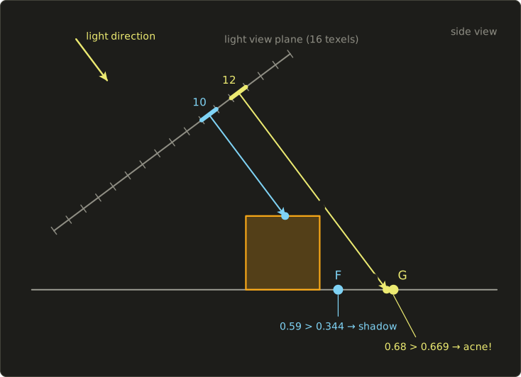
Now a floor point , well outside the shadow (the box top's shadow ends at ):
The center of row 12 is .
That ray misses the box and hits the floor at , , with and .
And now , so the test says shadow, although G is in plain sunlight!
Shadow acne and bias
What went wrong with G?
Each texel stores the depth of one sample, at its center, but the floor is tilted relative to the light, so its depth changes across the texel.
G lies 0.15 units (in ) past its texel's center, on the far side, so it is a little deeper than the sample: the floor shadows itself.
Over a whole surface, half of every texel is darker, which gives the typical stripes or moiré called shadow acne (シャドウアクネ):
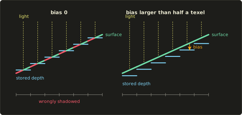
The usual fix is a depth bias (デプスバイアス): compare against a slightly larger value, .
How big must be?
On the floor, grows by per unit of (because and grows by ), and a point can be at most half a texel, units, from the center.
So the worst error is units, or in the 0 to 1 depth.
The factor is , where is the angle between the floor's normal and the direction to the light (): the more a surface is tilted away from the light, the more bias it needs.
Real renderers therefore use a slope-scaled bias, a constant plus a part proportional to the slope.
With , G gives : lit, as it should be.
Too much bias causes the opposite error.
Any receiver that is closer than to its occluder (measured along the light) is now treated as lit, so thin objects lose their shadow and the shadow of an object standing on the floor starts a little away from its base, as if the object floated.
This is called peter panning (ピーターパン現象), after Peter Pan, whose shadow comes loose.
Here is the whole story rendered with these formulas, the light of the worked example and a 48 × 48 shadow map:
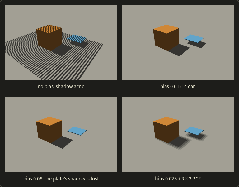
The plate floats 0.5 units above the floor, so along the light the gap is units, or in depth.
A bias of is larger than that, and the plate's shadow vanishes.
(The striped square in the first picture is exactly the area covered by the shadow map; outside it everything counts as lit.)
Resolution and aliasing
A shadow map is a sampled image, so everything from chapter 2 applies.
In our example a texel covers units, so a shadow edge can only move in steps of about half a unit: blocky, stair-stepped edges.
Worse, the shadow map's texels are spread evenly from the light's point of view, while the camera needs many more of them near itself, where one texel can cover dozens of pixels (perspective aliasing).
Typical remedies:
- higher shadow-map resolution (2048² or 4096² texels is common);
- fitting the light's frustum tightly around what the camera actually sees;
- cascaded shadow maps: several shadow maps for the sun, a detailed one for the area near the camera and coarser ones farther away.
Percentage-closer filtering
Can we blur the shadow map to soften the edges, like a texture?
Not directly: averaging depths doesn't give soft shadows.
Take a fragment with depth , bias , near a shadow edge, with these nine stored depths around it:
Their average is , and says "fully in shadow": still a yes-or-no answer, just at a wrong place.
Percentage-closer filtering (PCF, パーセンテージクローサーフィルタリング; Reeves, Salesin and Cook 1987) does the comparisons first and averages the results.
Here the four texels with pass () and the five with fail, so the point is lit: a value in between, which makes a soft edge.
GPUs support this in hardware: a "comparison sampler" (sampler2DShadow in GLSL, SamplerComparisonState in Slang and HLSL) compares and bilinearly filters four neighbors in one lookup.
PCF only blurs the edge by a fixed amount; it doesn't model a real penumbra that widens with distance from the occluder.
Methods that estimate the penumbra width (like percentage-closer soft shadows) are covered in Part 2.
Note in the fourth picture above that PCF needs a bit more bias (0.025 instead of 0.012), because it also compares against neighboring texels, whose centers are farther away.
Here are the lookup and a 3 × 3 PCF as shader functions.
The coordinates follow the OpenGL convention of the worked example; with Vulkan's depth range of 0 to 1, use ndc.z directly as the depth.
// Light-space lookup coordinates: (u, v) in the shadow map and the depth seen from the light.
float3 shadowCoords(float4x4 lightViewProj, float3 worldPos) {
  float4 clip = mul(lightViewProj, float4(worldPos, 1.0));
  float3 ndc = clip.xyz / clip.w;
  return float3(ndc.xy * 0.5 + 0.5, ndc.z * 0.5 + 0.5);
}

// 3 x 3 percentage-closer filtering: 1 = fully lit, 0 = fully in shadow.
float shadowPcf(Texture2D<float> shadowMap, SamplerState pointSampler, float3 uvDepth, float bias) {
  uint w, h;
  shadowMap.GetDimensions(w, h);
  float2 texel = float2(1.0 / float(w), 1.0 / float(h));
  float lit = 0.0;
  for (int y = -1; y <= 1; ++y) {
    for (int x = -1; x <= 1; ++x) {
      float stored = shadowMap.SampleLevel(pointSampler, uvDepth.xy + float2(x, y) * texel, 0);
      lit += (uvDepth.z - bias > stored) ? 0.0 : 1.0;
    }
  }
  return lit / 9.0;
}
// Light-space lookup coordinates: (u, v) in the shadow map and the depth seen from the light.
vec3 shadowCoords(mat4 lightViewProj, vec3 worldPos) {
vec4 clip = lightViewProj * vec4(worldPos, 1.0);
vec3 ndc = clip.xyz / clip.w;
return vec3(ndc.xy * 0.5 + 0.5, ndc.z * 0.5 + 0.5);
}
// 3 x 3 percentage-closer filtering: 1 = fully lit, 0 = fully in shadow.
float shadowPcf(sampler2D shadowMap, vec3 uvDepth, float bias) {
vec2 texel = 1.0 / vec2(textureSize(shadowMap, 0));
float lit = 0.0;
for (int y = -1; y <= 1; ++y) {
for (int x = -1; x <= 1; ++x) {
float stored = texture(shadowMap, uvDepth.xy + vec2(x, y) * texel).r;
lit += (uvDepth.z - bias > stored) ? 0.0 : 1.0;
}
}
return lit / 9.0;
}// Light-space lookup coordinates: (u, v) in the shadow map and the depth seen from the light.
float3 shadowCoords(float4x4 lightViewProj, float3 worldPos) {
float4 clip = mul(lightViewProj, float4(worldPos, 1.0));
float3 ndc = clip.xyz / clip.w;
return float3(ndc.xy * 0.5 + 0.5, ndc.z * 0.5 + 0.5);
}
// 3 x 3 percentage-closer filtering: 1 = fully lit, 0 = fully in shadow.
float shadowPcf(Texture2D<float> shadowMap, SamplerState pointSampler, float3 uvDepth, float bias) {
uint w, h;
shadowMap.GetDimensions(w, h);
float2 texel = float2(1.0 / float(w), 1.0 / float(h));
float lit = 0.0;
for (int y = -1; y <= 1; ++y) {
for (int x = -1; x <= 1; ++x) {
float stored = shadowMap.SampleLevel(pointSampler, uvDepth.xy + float2(x, y) * texel, 0);
lit += (uvDepth.z - bias > stored) ? 0.0 : 1.0;
}
}
return lit / 9.0;
}
The result multiplies the light's diffuse and specular terms (not the ambient term), so shadowed areas keep their ambient light.
You'll build the whole two-pass renderer yourself in the OpenGL series, chapter 23.
Why is shadow mapping the standard in real time?
It works for any geometry that can be rendered (no closed meshes or silhouettes needed), it handles self-shadowing and curved receivers, its cost hardly depends on scene complexity beyond one extra depth pass, and it can be filtered.
Its price is the bias tuning and the aliasing.
11.5 Ray-traced shadows and ambient occlusion
A ray tracer (chapter 12) answers "is this point hidden from the light?" in the most direct way: it shoots a shadow ray (シャドウレイ) from the point towards the light and checks whether anything is hit before the light.
For a point light at distance , the point is lit if no intersection exists with .
The small (or an offset of the ray's start along the normal) prevents the surface from hitting itself because of rounding errors: the ray-tracing version of shadow acne.
Shadow rays give exact hard shadows on anything, and they make soft shadows natural.
Replace the area light by many sample points and shoot one shadow ray to each.
Worked example. A point near a shadow edge sends 16 shadow rays to 16 points spread over an area light, and 6 of them are blocked: it gets of the light's direct contribution, so it lies in the penumbra.
With few rays the penumbra is noisy; how the noise shrinks with more rays is a topic of chapter 12 (Monte Carlo methods).
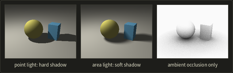
The third picture shows ambient occlusion (アンビエントオクルージョン, AO, 環境遮蔽).
The ambient term of chapter 10 assumes that light arrives equally from all directions at every point, which makes corners, creases and the ground under objects look flat and too bright.
Ambient occlusion measures how much of the hemisphere above a point is open: shoot rays into the hemisphere around the normal (up to some distance) and count how many escape.
Worked example: 32 rays, 8 hit nearby geometry, so the AO factor is and the ambient light at that point is multiplied by 0.75.
It's a cheap imitation of the darkening that full global illumination (chapter 12) would compute.
Film renderers compute it with rays, games approximate it from the depth buffer in screen space (SSAO, first shipped in Crysis in 2007) or bake it into textures; Part 2 goes deeper.
Comparing the shadow methods
| Method | Receivers | Self-shadowing | Soft shadows | Main cost and artifacts |
|---|---|---|---|---|
| Projected (planar) | one plane only | no | no (fake blur only) | cheap; z-fighting, anti-shadows above the light |
| Shadow volumes | everything | yes | no | silhouettes, closed meshes, fill rate; exact edges |
| Shadow mapping | everything | yes | with filtering (PCF) | extra depth pass; acne, peter panning, aliasing |
| Ray-traced shadows | everything | yes | yes, with area lights | many rays; noise in penumbrae |
Exam points
- 陰 (attached shadow, shade) comes from shading; 影 (cast shadow) needs a visibility test from the light.
- Point lights give hard shadows (umbra only); area lights give an umbra plus a penumbra.
- Projected shadows: a 4×4 matrix projects the object onto one plane from the light; no self-shadowing, no curved receivers.
- Shadow volumes: extrude silhouette edges, count crossings with the stencil buffer (front +1, back −1); nonzero means shadow. Z-pass breaks when the eye is inside a volume; z-fail fixes it with capped volumes.
- Shadow mapping: depth from the light, then compare. Acne → bias; too much bias → peter panning; limited resolution → aliasing; PCF compares first and averages after.
- Shadow rays: one ray per light (or per light sample); area lights → soft shadows.
11.6 Texture mapping and texture coordinates
Texture mapping (テクスチャマッピング) paints an image onto a surface.
Edwin Catmull described it in 1974, and it's the reason a 12-triangle box can look like a wooden crate.
Each pixel of a texture image is called a texel (テクセル), short for texture element, to keep it apart from the pixels of the screen.
Texture coordinates
To know which texel belongs to which point of the surface, every vertex gets texture coordinates (テクスチャ座標), usually written (UV座標).
They run from 0 to 1 across the image, whatever its size: is one corner, the opposite one.
Rasterization interpolates them across each triangle like any other vertex value (chapter 6), and the fragment shader reads the texture at the interpolated .
For a texture of texels, texel covers , and its center is at , exactly like the pixel centers of chapter 6.
(Which corner is, top or bottom of the image, differs between APIs and file formats; it's a frequent source of upside-down textures.)
Choosing texture coordinates for a surface is called parameterization (パラメータ化): a mapping from the 2D texture square onto the 3D surface.
For a parametric surface from chapter 8 it comes for free: its own parameters can serve directly as texture coordinates.
For a polygon mesh it has to be made, either by a simple projection or by unwrapping.
Projection mapping: planar, cylindrical, spherical, box
A quick way to get UVs is to project the texture onto the object from a simple shape.
Planar mapping (平面投影) projects along one axis, like a slide projector: for projection along z onto a rectangle from of size ,
It's perfect for flat things (a floor, a wall, a label) but smears the texture into streaks on surfaces parallel to the projection direction.
Cylindrical mapping (円筒投影) wraps the texture around an axis, here the y axis, with the angle around the axis as u:
( is the angle of the point , from −π to π, measured from +z towards +x.)
Worked example on a cylinder of radius 1 from to : the point has , so and .
The point on the front has and .
At the back, , gives , while a point just past it gives and : there's a seam where u jumps from 1 back to 0.
Spherical mapping (球面投影) uses longitude and latitude, like a world map:
Worked example: , a unit vector.
gives , and gives .
Besides the seam, spherical mapping has two poles: at the whole top row of the texture is squeezed into one point.
Box mapping (cube mapping of UVs, ボックス投影) uses six planar projections, one per side of a box, and picks for each point the one whose axis is closest to the surface normal (the largest component of the normal).
A point with normal uses the projection along y.
It avoids streaks, at the price of visible seams where two projections meet; blending the three projections smoothly is called triplanar mapping in game engines.
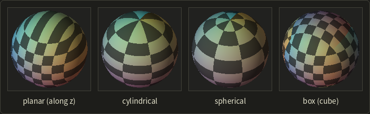
Look at the top of each sphere: planar mapping streaks, cylindrical mapping stretches the rows near the pole, spherical mapping pinches them into the pole, and box mapping keeps the squares square but has seams.
A classic generalization, two-part mapping (Bier and Sloan, 1986), first maps the texture onto such a simple intermediate shape and then transfers it to the real object, for example along the object's normals.
UV unwrapping and seams
For a character or a car, no single projection works.
Artists unwrap the mesh instead (UV展開): they cut it along chosen edges, the seams (継ぎ目, シーム), and flatten the pieces into the texture square, like the paper pattern of a piece of clothing.
The flattened pieces form a texture atlas; good unwrapping keeps the distortion (stretching) small and hides the seams where nobody looks.
A vertex on a seam has two different UVs, one for each side, so it must be stored twice, exactly like the split vertices of hard edges in chapter 9.
Wrap modes
What should happen for outside 0 to 1?
That's chosen by the wrap mode (ラップモード, also addressing mode):
- repeat (リピート): use the fractional part, , so the texture tiles. A floor with from 0 to 20 shows 20 tiles.
- clamp to edge (クランプ): clamp to , so the border texels are stretched outwards.
- mirrored repeat (ミラー): tile, but flip every second copy, so neighboring tiles meet without a jump.
Worked example. : repeat 0.3, clamp 1.0, mirror 0.3 (2 is even, no flip).
: repeat 0.8, clamp 0, mirror 0.2.
: repeat 0.3, clamp 1.0, mirror (1 is odd, flipped).
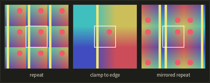
In OpenGL these are GL_REPEAT, GL_CLAMP_TO_EDGE and GL_MIRRORED_REPEAT, in Vulkan the VK_SAMPLER_ADDRESS_MODE_ values with the same names; a fourth option, clamp to border, returns a fixed border color outside.
11.7 Texture filtering
A texel almost never lands exactly on one pixel.
Either one texel covers several pixels, magnification (拡大): the camera is close or the texture is small.
Or one pixel covers several texels, minification (縮小): the surface is far away or seen at a grazing angle.
These two cases need different filters.
Magnification: nearest and bilinear
Nearest-neighbor sampling (最近傍補間, ニアレストネイバー) takes the texel that contains the point: , .
It's fast and keeps hard pixel edges (pixel-art games want exactly that), but a magnified texture turns into visible blocks.
Bilinear interpolation (双線型補間, バイリニア補間) blends the four texels whose centers surround the point.
Shift the coordinates so that texel centers land on whole numbers,
then interpolate linearly along x in both rows, and once along y between the two results:
Worked example. A 4 × 4 gray texture with , , , , sampled at :
So , , , :
Nearest sampling gives , , so .
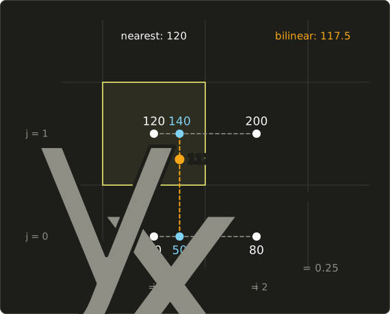
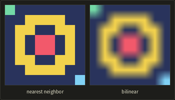
Bilinear magnification is smooth but blurry; it can't invent detail that isn't in the texture.
Higher-order filters such as bicubic interpolation (双三次補間) use 4 × 4 texels and are sharper; they come back with image resampling in chapter 15.
Here are the two samplers and the wrap modes in C++:
#include <cmath>
#include <cstdio>

enum class Wrap { Repeat, Clamp, Mirror };

// Maps any texture coordinate into [0, 1] with the chosen wrap mode.
float wrap(float u, Wrap mode) {
  float k = std::floor(u);
  float f = u - k;
  switch (mode) {
  case Wrap::Repeat: return f;
  case Wrap::Clamp: return std::fmin(std::fmax(u, 0.0f), 1.0f);
  case Wrap::Mirror: return (static_cast<long>(k) % 2 == 0) ? f : 1.0f - f;
  }
  return f;
}

// A gray texture of w x h texels, row 0 first.
struct Texture {
  int w, h;
  const float *texels;
  float at(int i, int j) const { // texel (i, j), clamped to the edge
    i = i < 0 ? 0 : (i >= w ? w - 1 : i);
    j = j < 0 ? 0 : (j >= h ? h - 1 : j);
    return texels[j * w + i];
  }
};

float sampleNearest(const Texture &t, float u, float v) {
  return t.at(static_cast<int>(std::floor(u * t.w)), static_cast<int>(std::floor(v * t.h)));
}

float sampleBilinear(const Texture &t, float u, float v) {
  float x = u * t.w - 0.5f, y = v * t.h - 0.5f; // texel centers sit on whole numbers
  int i = static_cast<int>(std::floor(x)), j = static_cast<int>(std::floor(y));
  float fx = x - i, fy = y - j;
  float a = t.at(i, j) + fx * (t.at(i + 1, j) - t.at(i, j));             // along the row j
  float b = t.at(i, j + 1) + fx * (t.at(i + 1, j + 1) - t.at(i, j + 1)); // along the row j + 1
  return a + fy * (b - a);
}

// Mip level from the texel-space footprint of one pixel step in x and in y.
float mipLevel(float dudx, float dvdx, float dudy, float dvdy) {
  float rho = std::fmax(std::sqrt(dudx * dudx + dvdx * dvdx), std::sqrt(dudy * dudy + dvdy * dvdy));
  return std::log2(rho);
}

int main() {
  const float texels[16] = {0, 40, 80, 0,     // row j = 0
                            0, 120, 200, 0,   // row j = 1
                            0, 0, 0, 0,       // row j = 2
                            0, 0, 0, 0};      // row j = 3
  Texture tex{4, 4, texels};
  printf("nearest  %g\n", sampleNearest(tex, 0.4375f, 0.3125f));
  printf("bilinear %g\n", sampleBilinear(tex, 0.4375f, 0.3125f));
  const float us[3] = {2.3f, -0.2f, 1.3f};
  for (float u : us) {
    printf("u = %4.1f: repeat %.1f, clamp %.1f, mirror %.1f\n", u, wrap(u, Wrap::Repeat),
           wrap(u, Wrap::Clamp), wrap(u, Wrap::Mirror));
  }
  printf("mip level %g\n", mipLevel(4, 0, 0, 8));
  return 0;
}
nearest  120
bilinear 117.5
u =  2.3: repeat 0.3, clamp 1.0, mirror 0.3
u = -0.2: repeat 0.8, clamp 0.0, mirror 0.2
u =  1.3: repeat 0.3, clamp 1.0, mirror 0.7
mip level 3
Minification and mipmaps
Minification is the dangerous case.
If one pixel covers 8 × 8 texels and we read only one or four of them, we are sampling the texture far below its Nyquist frequency: a fine pattern turns into moiré, and in motion it shimmers.
That's exactly the aliasing of chapter 2 (section 2.6).
The honest fix is pre-filtering (section 2.7): average all the texels under the pixel.
Doing that for every pixel at run time would be far too slow, so we do it once, in advance.
A mipmap (ミップマップ, Lance Williams 1983; "mip" is Latin multum in parvo, "much in a small space") stores the texture together with a chain of smaller copies.
Level 0 is the original, and each next level halves the width and height, every texel being the average of 2 × 2 texels of the level above, down to 1 × 1.
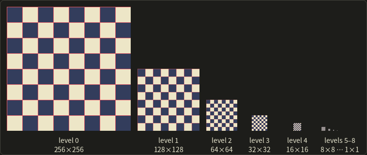
Memory, worked. A 1024 × 1024 RGBA texture with 8 bits per channel takes bytes, 4 MiB.
It has levels (1024, 512, …, 1).
Each level has a quarter of the texels of the one before, so all levels together take
times the original: bytes, about 5.33 MiB, only a third more.
Choosing the level.
The GPU measures how far the texture coordinates move between neighboring pixels: the derivatives for one pixel to the right and for one pixel down, multiplied by the texture size so that they're in texels.
The pixel's footprint (フットプリント) in the texture is roughly a parallelogram spanned by these two vectors, and its size is
The level is the one where one texel is about as big as the footprint.
Worked example. A floor seen at an angle: one pixel to the right moves 4 texels in u, one pixel down moves 8 texels in v.
So and : level 3, a 128 × 128 texture, where one texel covers 8 × 8 original texels.
(GPUs compute these derivatives by comparing neighboring pixels in 2 × 2 blocks, which is why they are available in fragment shaders as dFdx/dFdy in GLSL and ddx/ddy in Slang and HLSL.)
For magnification , and the GPU switches to the magnification filter on level 0.
Trilinear filtering (トライリニアフィルタリング).
is rarely a whole number.
Bilinear filtering on the nearest level would make visible bands where the level jumps, so trilinear filtering samples the two nearest levels bilinearly and blends them: for , half of level 2 and half of level 3.
That's 8 texel reads per sample.
Anisotropic filtering (異方性フィルタリング).
In the example the footprint is twice as long in v as in u.
Choosing the level from the longer side (8 texels) blurs the short direction too much, so floors and roads at grazing angles get muddy.
Anisotropic filtering takes several samples along the long axis, each from a sharper level chosen by the short side.
Here: samples from level , spread along v.
GPUs allow up to 16 samples ("16× anisotropic").
(An older alternative to mipmaps, the summed-area table of Crow 1984, can average any axis-aligned rectangle in constant time.)
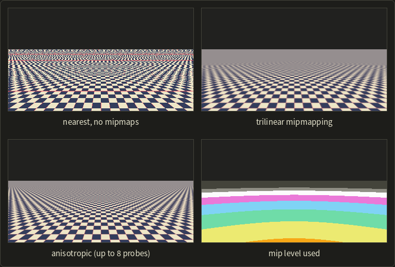
Without mipmaps the distance dissolves into noise and moiré; trilinear mipmapping replaces it with the correct average (gray) but turns the floor blurry early; anisotropic filtering keeps the squares sharp much farther.
The fourth picture colors each pixel by the level it uses, red, orange, yellow, green, blue, pink and white for levels 0 to 6: the farther away, the smaller the level's texture.
In the GLSL series, chapter 11 and the OpenGL series, chapter 6 you'll set these filter modes yourself.
Perspective-correct texture coordinates
Section 6.9 of chapter 6 warned that interpolating with screen-space weights is wrong under perspective.
For textures you can see the error: straight lines of the texture bend and swim.
Worked example. An edge goes from a vertex with and to a vertex with and (w is the distance in front of the camera, chapter 6).
At the screen midpoint, plain interpolation gives .
The perspective-correct way interpolates and linearly on the screen and divides:
The middle of the screen shows the texture at , not 0.5, because the near part of the edge takes up more of the screen.
GPUs do this automatically.
The first PlayStation (1994) famously didn't, which is why its textures wobble when the camera moves.
Exam points
- Magnification → nearest or bilinear; minification → mipmaps (plus trilinear or anisotropic filtering).
- Bilinear uses the 4 nearest texels; trilinear blends bilinear results of 2 mip levels (8 texels).
- A mipmap pyramid costs about 1/3 extra memory; each level halves the size; the level is of the footprint in texels.
- Mipmapping is pre-filtering against aliasing; it does not improve magnification.
- Texture coordinates must be interpolated perspective-correctly.
- Projection mappings: planar (streaks), cylindrical (seam), spherical (seam and poles), box (seams between faces).
11.8 Bump, normal, displacement and parallax mapping
A texture doesn't have to hold colors.
It can hold anything a shader uses per point, and some of the most useful ones change the shape that lighting sees.
Bump mapping
James Blinn's bump mapping (バンプマッピング, 1978) keeps the geometry smooth and only tilts the normal used for lighting, as if the surface had small bumps.
The bumps come from a height map (高さマップ) , a gray texture where bright means high.
For a flat piece of surface with normal and the texture's u and v along x and y, a surface raised by has the normal
(the normal tilts away from the uphill direction, like the side of a hill).
On a curved surface the same happens in the surface's own frame: , with and the unit directions of u and v on the surface (the tangent space of the next section).
The slopes come from neighboring texels, for example with central differences.
Worked example. Around one texel the heights are 0.2 to the left and 0.5 to the right, 0.3 below and 0.3 above, with a texel spacing of 1:
With the light direction (from the left), the flat surface gets the diffuse factor , the bumped one : the slope facing the light is brighter.
With the light from the right, , it gets , darker.
That light-and-dark pattern is all the eye needs to see a bump.
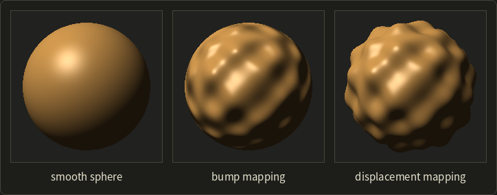
Compare the outlines in the middle and on the right.
Bump mapping changes only the lighting, so the silhouette stays a perfect circle, the bumps cast no shadows and don't hide each other.
That's the giveaway of bump mapping at grazing angles.
Normal mapping and tangent space
Normal mapping (法線マッピング) stores the perturbed normal itself instead of the height, so the shader doesn't need to compute slopes.
A normal has components from −1 to 1, and a color channel holds 0 to 1 (0 to 255 in 8 bits), so each component is stored as and decoded as
Worked example. The texel in 8 bits is and decodes to
whose length is 1.003, so after normalizing it's about : a normal tilted towards +u.
An untilted normal is stored as , a light blue-violet, which is why normal maps look mostly blue.
The normals in such a map are given in tangent space (接空間, タンジェント空間): a frame that sits on the surface with (tangent) along the direction of increasing u, (bitangent) along increasing v and the surface normal.
That way one brick texture works on every wall, whatever its orientation.
The shader turns a tangent-space normal into world space with the TBN matrix, whose columns are the three vectors:
The tangent comes from the triangle's positions and UVs.
With edges , and UV differences , :
Worked example. A floor triangle , , with UVs , , .
Then , , , , , , the denominator is 1, and , , normalized and .
(Linear Algebra chapter 5), the floor's normal, so the frame is right-handed.
The decoded normal becomes in world space: tilted towards +x.
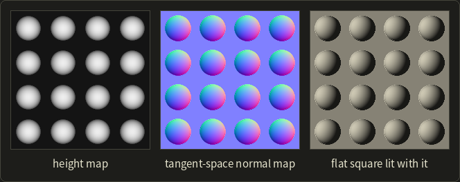
In the normal map, the right sides of the studs are reddish (), the upper sides greenish (), and the flat background is the typical blue.
Normal maps are usually baked from a detailed sculpt onto a low-polygon model: the game model has a few thousand triangles, but lights it as if it had millions.
Remember from chapter 3 that a normal map holds data, not colors, so it must not be decoded as sRGB.
In a shader the decoding and the TBN transform are only two lines:
// Tangent-space normal from a normal-map texel (components in [0, 1]) to world space.
float3 normalFromMap(float3 texel, float3 T, float3 B, float3 N) {
  float3 n = normalize(texel * 2.0 - 1.0);
  return normalize(n.x * T + n.y * B + n.z * N);
}
// Tangent-space normal from a normal-map texel (components in [0, 1]) to world space.
vec3 normalFromMap(vec3 texel, vec3 T, vec3 B, vec3 N) {
vec3 n = normalize(texel * 2.0 - 1.0);
return normalize(n.x * T + n.y * B + n.z * N);
}// Tangent-space normal from a normal-map texel (components in [0, 1]) to world space.
float3 normalFromMap(float3 texel, float3 T, float3 B, float3 N) {
float3 n = normalize(texel * 2.0 - 1.0);
return normalize(n.x * T + n.y * B + n.z * N);
}You'll implement normal mapping in the GLSL series, chapter 12 and the OpenGL series, chapter 22.
Displacement mapping
Displacement mapping (ディスプレイスメントマッピング, Cook 1984) really moves the surface: each point is pushed along its normal by the height,
with a scale .
Because the geometry changes, the silhouette, the shadows and the occlusion are all correct (the right sphere above).
The price: the surface must be finely subdivided so that there are vertices to move, at least one per bump.
Film renderers subdivide down to pixel-sized micropolygons; GPUs use tessellation shaders to create the extra vertices on the fly.
Parallax mapping
Parallax mapping (視差マッピング, Kaneko et al. 2001) sits between the two.
When you look at a bumpy surface at an angle, the raised parts appear shifted towards you.
Parallax mapping imitates that by shifting the texture coordinates before reading the textures:
where is the direction to the eye in tangent space.
Worked example. , height , scale : the shift is in u.
The flatter the viewing angle (small ), the larger the shift.
Parallax occlusion mapping refines this by marching along the view ray through the height field, which also lets bumps hide each other; the silhouette, however, stays flat.
11.9 Environment mapping
Shiny surfaces reflect their surroundings.
Tracing real reflection rays is the job of chapter 12; environment mapping (環境マッピング, also reflection mapping, Blinn and Newell 1976) fakes it with a texture.
The idea: store an image of the surroundings as seen from one point, in all directions.
To shade a point of a mirror-like object, compute the reflection vector of the view direction and look up the environment in that direction.
With the incident direction (from the eye to the surface) and the unit normal :
This is GLSL's, Slang's and HLSL's reflect(I, n), built from the dot product of Linear Algebra chapter 4.
Worked example. The eye looks straight down −z, , at a surface with :
The reflection goes mostly up, so this point shows the sky.
(Its length is , as a reflection of a unit vector should be.)
Cube maps
A cube map (キューブマップ, cubic environment map, Greene 1986) stores the surroundings on the six faces of a cube around the point: +X, −X, +Y, −Y, +Z and −Z, each a normal square texture rendered with a 90° camera.
To look up a direction, take its component with the largest absolute value: that picks the face, and dividing by it gives the position on that face.
For the largest component is , so it's the +Y face, and is the point where the ray pierces the cube.
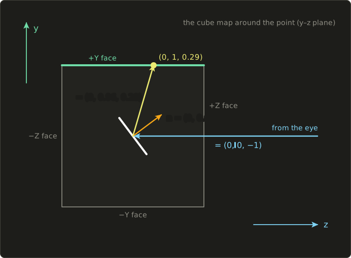
Cube maps have almost even resolution in all directions, can be rendered by the GPU itself (six renders, even every frame for a dynamic reflection), and have been supported in GPU hardware since around 2000.
They're today's standard; the OpenGL series, chapter 18 uses them for a sky box and reflections.
Sphere maps and latitude–longitude maps
A sphere map (スフィアマップ, 球面環境マップ) is one image of a perfectly mirroring ball, photographed (or rendered) from far away.
The classic fixed-function OpenGL formula (GL_SPHERE_MAP) maps a reflection vector in eye space to
Worked example with our : , so and .
The direction straight back at the eye, , lands in the center (, ), and the direction straight away from the eye, , gives : it's smeared around the whole rim.
A sphere map is therefore tied to one viewing direction and has poor resolution at the rim; that's why cube maps replaced it.
The third common format is the latitude–longitude (equirectangular) map, which is just the spherical mapping of section 11.6 applied to directions; HDR environment photos (light probes) are usually stored that way, and chapter 12 uses them for image-based lighting.
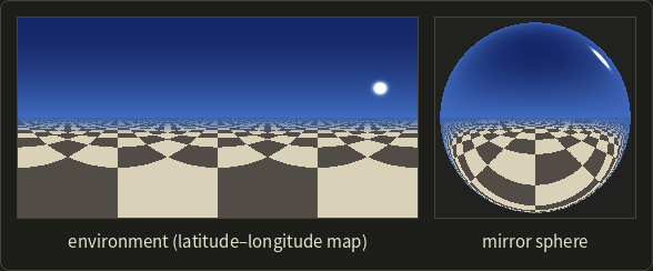
Limits and refraction
Environment mapping assumes the surroundings are infinitely far away: the lookup depends only on the direction of , not on where the reflecting point is.
So reflections of nearby objects are in the wrong place, an object can't reflect itself, and two shiny objects don't reflect each other correctly (unless you render a separate map per object, and even then only approximately).
Real-time renderers improve this with several local maps (reflection probes) and screen-space reflections; exact reflections need ray tracing (chapter 12).
The same lookup works for refraction (屈折): bend the view vector with Snell's law (refract(I, n, eta) in GLSL, Slang and HLSL) instead of reflecting it, and look up the environment behind a glass object; Snell's law itself is in chapter 12.
11.10 More kinds of maps
The texture lookup is so cheap that almost every material parameter has its own map.
Specular and other material maps.
A specular (gloss) map sets the shininess or the strength of the highlight per texel: wet patches shine, dry ones don't.
Physically based renderers use roughness and metallic maps the same way (Part 2); you'll use lighting maps in the OpenGL series, chapter 11.
Light maps (ライトマップ).
For static scenes, lighting (including soft shadows and indirect light) can be computed once, offline, and stored in a second, low-resolution texture over the whole level.
At run time the color is just : a wall texel with albedo 0.8 in a spot where the light map says 0.5 is drawn as 0.4.
Quake (1996) made light maps famous, and "baked lighting" is still standard for static parts of game levels.
The price: the light can't move, and every surface needs its own non-overlapping UVs for the light map.
Alpha maps and cut-outs (アルファマップ, 透明度マップ).
The alpha channel of a texture can hold opacity.
For leaves, grass, fences and hair, a simple quad with an alpha map shows a complex outline: with alpha testing the fragment shader discards fragments whose alpha is below a threshold (say 0.5), which needs no sorting; semi-transparent glass uses alpha blending, whose order problems are discussed in chapter 10.
Projective texture mapping (投影テクスチャマッピング, Segal et al. 1992).
Here texture coordinates aren't stored on the vertices but computed like a slide projector: transform the point with a projector's view and projection matrices and use the resulting , exactly the of section 11.4.
That's how a flashlight projects a cookie pattern or a car's headlights show their shape on a wall.
Shadow mapping is the same lookup with a depth comparison added.
Solid textures and procedural textures
A 2D texture is glued onto the surface, which shows when you cut an object: a wooden block made of six textured faces doesn't look like it was carved from wood.
A solid texture (ソリッドテクスチャ, 3D texture; Perlin 1985, Peachey 1985) is a function of the 3D position instead, so the object is "carved" out of the material and needs no UVs at all.
Storing it as a 3D image costs a lot of memory ( texels at 4 bytes are 64 MiB), so it's usually computed: a procedural texture (プロシージャルテクスチャ) is a short program that computes the color from the position.
- Wood: rings around an axis, , mapped to light and dark wood colors.
- Marble: veins, , mapped to white and gray.
Both need noise (ノイズ関数): a random-looking but smooth function.
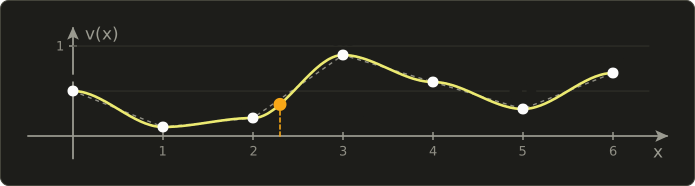
The simplest is value noise: give each integer lattice point a random value and interpolate smoothly between them.
In 1D with lattice values , for between and :
The "smoothstep" curve has zero slope at both ends, so the curve has no kinks at the lattice points.
Worked example. With and , at : , , and .
Plain linear interpolation would give .
Perlin noise (パーリンノイズ) stores a random gradient (a slope direction) at each lattice point instead of a value, which avoids the blocky look of value noise; its value at the lattice points is 0.
Adding several octaves of noise, each with double the frequency and half the amplitude, gives fractal noise or fBm, and summing the absolute values gives turbulence (乱流), which Perlin used for marble, clouds and fire.
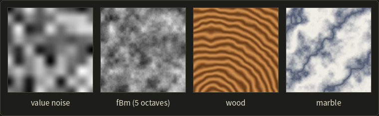
Procedural textures need almost no memory, have unlimited resolution and never repeat, but they cost computation per sample and are hard to filter (they alias when minified, since there's no mipmap).
You'll write noise functions yourself in the GLSL series, chapter 8.
Exam points
- Bump mapping: perturbs normals from a height map; geometry and silhouette unchanged.
- Normal mapping: stores the normal (usually in tangent space, decoded with and the TBN matrix).
- Displacement mapping: moves the geometry; the silhouette changes; needs fine tessellation.
- Environment mapping: look up the surroundings with the reflection vector ; sphere map (one image, view-dependent) vs cube map (six faces); assumes distant surroundings, no self-reflection.
- Solid textures are functions of 3D position (wood, marble); procedural noise (Perlin) makes them look natural.
- Light maps store precomputed lighting; projective textures compute UVs from a projector's matrices.
11.11 Summary
- A point is in shadow when it is hidden from the light; attached shadows (陰) come from shading, cast shadows (影) from a visibility test from the light.
- Point lights give hard shadows; area lights give an umbra and a penumbra whose width grows with the distance from the occluder.
- Projected shadows flatten the object onto a plane with the matrix ; cheap, but only for one flat receiver.
- Shadow volumes extrude silhouette edges and count crossings in the stencil buffer (z-pass, or z-fail when the eye can be inside).
- Shadow mapping renders depth from the light and compares; bias fights acne, too much bias causes peter panning, PCF softens edges by averaging comparison results.
- Shadow rays test visibility directly; with area lights they give soft shadows; ambient occlusion darkens enclosed places.
- Texture coordinates map the texture square onto the surface (planar, cylindrical, spherical, box projection or unwrapping); wrap modes handle coordinates outside 0 to 1.
- Magnification uses nearest or bilinear filtering; minification needs mipmaps (1/3 extra memory, level ), trilinear and anisotropic filtering; interpolation must be perspective-correct.
- Bump and normal mapping change the lighting normal, displacement mapping the geometry, parallax mapping the texture coordinates.
- Environment maps (cube maps, sphere maps) fake reflections and refractions of distant surroundings; light maps, alpha maps, projective and procedural (solid) textures complete the toolbox.
11.12 Key terms
| English | 日本語 |
|---|---|
| shadowing | 影付け |
| attached shadow, shade | 陰 |
| cast shadow | 影 |
| self-shadowing | セルフシャドウ |
| umbra | 本影 |
| penumbra | 半影 |
| hard shadow, soft shadow | ハードシャドウ、ソフトシャドウ |
| projected (planar) shadow | 投影法(平面への投影による影) |
| shadow volume | シャドウボリューム法 |
| silhouette edge | シルエットエッジ(輪郭エッジ) |
| stencil buffer | ステンシルバッファ |
| depth pass, depth fail | Zパス法、Zフェイル法 |
| shadow mapping, shadow map | シャドウマッピング、シャドウマップ |
| shadow acne | シャドウアクネ |
| depth bias | デプスバイアス |
| peter panning | ピーターパン現象 |
| percentage-closer filtering (PCF) | PCF(パーセンテージクローサーフィルタリング) |
| shadow ray | シャドウレイ |
| ambient occlusion | アンビエントオクルージョン(環境遮蔽) |
| texture mapping | テクスチャマッピング |
| texel | テクセル |
| texture coordinates (UV) | テクスチャ座標(UV座標) |
| parameterization | パラメータ化 |
| planar, cylindrical, spherical, box mapping | 平面投影、円筒投影、球面投影、ボックス投影 |
| UV unwrapping, seam | UV展開、継ぎ目(シーム) |
| wrap mode (repeat, clamp, mirror) | ラップモード(リピート、クランプ、ミラー) |
| magnification, minification | 拡大、縮小 |
| nearest-neighbor interpolation | 最近傍補間(ニアレストネイバー) |
| bilinear interpolation | 双線型補間(バイリニア補間) |
| mipmap | ミップマップ |
| trilinear filtering | トライリニアフィルタリング |
| anisotropic filtering | 異方性フィルタリング |
| bump mapping | バンプマッピング |
| height map | 高さマップ |
| normal mapping | 法線マッピング |
| tangent space | 接空間(タンジェント空間) |
| displacement mapping | ディスプレイスメントマッピング |
| parallax mapping | 視差マッピング(パララックスマッピング) |
| environment (reflection) mapping | 環境マッピング(反射マッピング) |
| cube map, sphere map | キューブマップ、スフィアマップ(球面環境マップ) |
| light map | ライトマップ |
| alpha map | アルファマップ(透明度マップ) |
| projective texture mapping | 投影テクスチャマッピング |
| solid texture | ソリッドテクスチャ(3次元テクスチャ) |
| procedural texture | プロシージャルテクスチャ |
| noise function, Perlin noise | ノイズ関数、パーリンノイズ |
11.13 Challenges
- ★ Build the shadow matrix for the plane and a point light at , and project the points and . Then project and explain what goes wrong.
- ★ A 2 × 2 gray texture has , , , . With clamp to edge, compute the nearest and the bilinear sample at and at . Which coordinates do and become with repeat, clamp and mirrored repeat?
- ★★ Compute the cylindrical (with y from −1 to 1) and the spherical texture coordinates (formulas of section 11.6) of the unit vectors and . Which of the two lies on the seam, and what would a triangle that straddles the seam look like if its vertices kept their computed u values?
- ★★ A wall faces +z with , , . Decode the normal-map texel , transform it to world space, and compare the diffuse factor of the flat and the normal-mapped wall for and for .
- ★★★ A shadow map is sampled with bilinear filtering of the stored depths before the comparison. Using a 1D row of four texels with depths 0.3, 0.3, 0.9, 0.9 and a receiver at depth 0.7 moving from the first to the last texel, show what the shadow looks like, and compare with comparing first and averaging after (PCF). Why can't depth averaging ever produce a penumbra?
Multiple choice
Q1 ★ Which of the following statements about shadow generation is correct?
| A | Shadow mapping first renders the depths of the scene from the light, and then, while rendering from the camera, compares each point's depth seen from the light with the stored depth. |
| B | The projected (planar) shadow method can cast shadows onto curved surfaces and onto the object itself. |
| C | The shadow volume method decides shadows without counting how many faces of the volumes a ray crosses. |
| D | A point light produces a wide penumbra around every shadow. |
| E | Shadow mapping is free of aliasing, because the depth comparison is exact. |
Q2 ★ Which of the following statements about mapping techniques is correct?
| A | Bump mapping moves the vertices of the surface along their normals. |
| B | Normal mapping changes the silhouette of an object. |
| C | Environment mapping correctly reflects nearby objects, including the object itself. |
| D | Displacement mapping actually moves the surface, so the silhouette and the shadows change too. |
| E | A tangent-space normal map stores heights as gray values. |
Q3 ★★ A 1024 × 1024 texture is used with a full mipmap. Which of the following statements is correct?
| A | Mipmapping is mainly used to improve the quality of magnification. |
| B | All levels together need about twice the memory of the original texture. |
| C | Including the original, the mipmap has 10 levels. |
| D | Trilinear filtering blends nearest-neighbor samples from four neighboring levels. |
| E | The level is chosen from the size of a pixel's footprint in texels; a footprint of about 8 texels selects level 3, a 128 × 128 texture. |
11.14 Practical assignment
Build a tiny shadow map and a tiny mipmap by hand, and check both against exact answers.
You need graph paper, a ruler, a pencil, two colored pens and a calculator.
Part A: a shadow map in a side view.
The scene is 2D (x to the right, y up): the floor from to and a box from to , to .
Sunlight travels in the direction .
As light-space coordinates use (across the light) and the depth (along the light: a smaller z is nearer to the sun).
- Draw the scene at 1 unit = 2 cm, with a few parallel light rays.
- Exact shadow. Project the box's top corners onto the floor along (a point lands at ). Which interval of the floor is in shadow? Mark it with the first pen.
- Fill the shadow map. The map has 5 texels of width 1 in s, covering . For each texel center , find the first surface the light reaches on the line (floor, the box's left side or its top ; the hit with the smallest z wins) and write down its depth.
- Test the floor. For the floor points , compute s, the texel, and z, and compare with the stored depth (shadow when ). Mark the points that come out in shadow with the second pen. Which point is wrongly shadowed (acne), and why?
- Bias. Show that a floor point can be up to half a texel from its texel center and that this changes its depth by at most . Repeat step 4 with the test .
Part B: a mipmap by hand.
A 4 × 4 gray texture (row first): 20, 60, 100, 140 / 60, 20, 140, 100 / 100, 140, 20, 60 / 140, 100, 60, 20.
- Build the pyramid. Compute level 1 (2 × 2, each texel the average of a 2 × 2 block) and level 2 (1 × 1).
- Bilinear on two levels. Sample bilinearly on level 0 (4 × 4) and on level 1 (2 × 2), using , with the size of that level.
- Choose and blend. One pixel step moves the coordinates by texels in x and by texels in y (level-0 texels). Compute and , and the trilinear result as the blend of your two bilinear results.
How to check yourself:
- Part A: the exact shadow is (step 2); with the bias, the shadow-map test must agree with it for every test point; without the bias exactly one test point is wrong, and it lies in the far half of its texel.
- Part A: the stored depth of the texel that sees only the floor equals of the floor point on its center line.
- Part B: level 2 equals the average of all 16 texels; each bilinear result lies between the smallest and the largest of the four texels it used; the trilinear result lies between the two bilinear results, exactly in the middle when .
コメント(0)
まだコメントはありません。
ログインするとコメント出来ます。