21. Mesh Processing and Signed Distance Fields
In Part 1 we met two ways to describe a surface: as a polygon mesh (chapter 9, with its topology from chapter 7) and as an implicit function .
This chapter is about working with both.
For meshes, that means the algorithms that modeling tools, game engines and 3D scanners run behind the scenes: smoothing a noisy scan, simplifying a model for LOD, repairing broken geometry, flattening a surface for its UV layout, and baking detail into normal maps.
For implicit surfaces, it means the signed distance field (符号付き距離場, SDF): we'll see why sphere tracing can't miss a surface, blend shapes smoothly, compute SDFs from meshes, draw sharp text from tiny textures, and turn SDFs back into meshes.
Hardly any mesh in a game or a film is drawn as it was first built, and SDFs have become part of real-time engines, for soft shadows, global illumination, collisions and text.
Chapter 9 promised two things for Part 2: the derivation of the quadric error metric for simplification, and a proper treatment of SDFs; here they are.
This goes beyond the exam syllabus, but it deepens three of its items: polygon surfaces (ポリゴン曲面の表現), implicit surfaces and marching cubes, and texture mapping.
The math needs dot and cross products and small matrices from the Linear Algebra series, plus gradients, which I'll explain as we go.
21.1 Meshes as discrete surfaces
A smooth surface has normals, curvature and a Laplace operator at every point; a triangle mesh only has vertices, edges and flat faces.
Discrete differential geometry (離散微分幾何) defines mesh versions of these quantities that behave like the smooth ones and become exact as the mesh gets finer.
Most mesh algorithms are built from two of them: a Laplacian and a curvature.
Both look at a vertex's one-ring (1-リング近傍): its neighbors (the vertices joined to it by an edge) and the faces around it, exactly what the half-edge structure of chapter 7 lets you walk around.
The number of neighbors is the valence (価数), 6 in a regular triangle mesh.
The discrete Laplacian: the umbrella operator
The simplest discrete Laplacian compares a vertex with the average of its neighbors:
It's called the umbrella operator (アンブレラ演算子), because the neighbors spread around the vertex like the ribs of an umbrella; is their centroid:
It's the mesh version of the Laplacian filter of chapter 15 (section 15.5), which compared a pixel with its four neighbors.
On a flat, regular patch ; on a bump, points into the bump, roughly along the normal.
Worked example. A vertex sits 0.3 above a flat floor, with four neighbors , , and .
The centroid is , so : straight down, the height of the bump.
The umbrella operator ignores the shape of the triangles, so on an irregular mesh it also pulls vertices sideways.
The geometrically correct version weights neighbor with the cotangent weights (コタンジェント重み, Pinkall and Polthier, 1993) , where and are the two angles opposite the edge .
Then points exactly along the normal, and its length (divided by the vertex's area) approximates twice the mean curvature (平均曲率), the average bending of the surface.
Curvature from angles: the angle defect
Lay the faces around a vertex flat on a table.
On a flat surface their corners add up to 360° and they lie flat without a gap.
At the corner of a cube, three right angles add up to only 270°, leaving a 90° gap; at a saddle there's too much angle, and the paper would have to wrinkle:
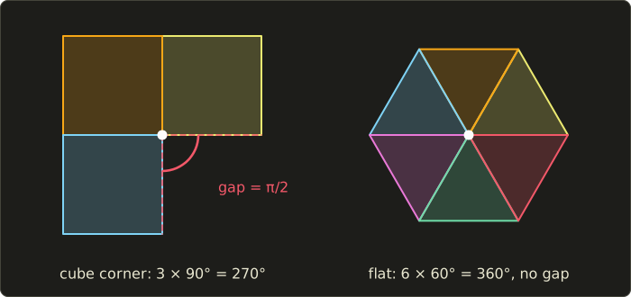
That missing angle is the angle defect (角度欠損), the discrete Gaussian curvature (ガウス曲率) concentrated at the vertex:
where is the corner angle of face at the vertex.
Positive means sphere-like, zero means flat or bent in one direction only (a cylinder unrolls flat), negative means saddle-like.
- Cube corner: (90°).
- Octahedron vertex, four equilateral triangles: (120°).
- Flat grid vertex, six equilateral triangles: .
- Saddle where five squares meet: .
Now add up a whole closed mesh: the cube's 8 corners give , the octahedron's 6 vertices .
That's Descartes' theorem, the discrete Gauss–Bonnet theorem (ガウス・ボネの定理):
and for every closed mesh without holes (Euler's formula, chapter 7).
The total curvature is a topological constant: moving vertices moves curvature around, but can't create or destroy it.
A torus () has total curvature 0: positive outside, negative inside.
In practice the angle defect is used to find sharp corners, detect noise in scans, and paint the "curvature maps" texture artists use for edge wear.
21.2 Smoothing and fairing
A 3D scan, a marching cubes surface or a photogrammetry mesh is always a little noisy.
Smoothing (平滑化, also fairing, フェアリング) removes the high-frequency bumps and keeps the overall shape, like a blur filter on an image.
Laplacian smoothing
Move every vertex a fraction of the way towards the centroid of its neighbors, all at the same time (compute all new positions from the old ones, then replace them), and repeat:
That's Laplacian smoothing (ラプラシアンスムージング).
In the example above, moves the bump vertex to : one step halves the bump.
Why it shrinks
Laplacian smoothing has a famous flaw: everything shrinks, not only the noise.
Take a clean regular octagon of radius 1, each point with two neighbors 45° away.
Their average lies on the same ray from the center at distance , so the umbrella vector points to the center with length , and one step with shrinks the radius to
After 10 steps the radius is : a fifth of the original, although there was no noise at all.
The frequency view explains it.
On a closed loop of points, the shapes (point , frequency ) are only scaled by the umbrella operator, by with
so one smoothing step multiplies frequency by .
The octagon's circle is the lowest frequency , with as computed.
The noisiest shape, a zigzag (every other point pushed out), has and is multiplied by : with it disappears in one step.
So Laplacian smoothing is a low-pass filter (ローパスフィルタ), but a leaky one: every frequency except (moving the whole shape) is damped, and the shape shrinks with the noise.
Taubin's λ|μ smoothing
Taubin (1995) fixed this with a second step: after each shrinking step with , take an inflating step with a negative :
One pair multiplies frequency by
which equals 1 at and again at the pass-band frequency (通過帯域周波数)
Below the shape passes (in fact is very slightly above 1 there), above it bumps are damped.
Taubin recommends between 0.01 and 0.1, and his examples use with , which gives ().
| meaning | Laplacian, | Taubin pair | |
|---|---|---|---|
| 0.0192 | circle on a 32-gon | 0.9904 | 1.0007 |
| 0.2929 | circle on an octagon | 0.8536 | 0.9760 |
| 1 | medium noise | 0.5 | 0.6179 |
| 2 | zigzag | 0 | −0.6134 |
For example, at : .
A finely sampled circle survives, while a zigzag loses about 40% per pair (the minus sign means it flips each time).
The octagon is so coarse that its "circle" already counts as high frequency, so even Taubin shrinks it a little.
For a 32-point circle with a zigzag of , 20 Laplacian steps remove the zigzag and shrink the radius to ; 20 Taubin pairs remove the zigzag too and keep the radius ().
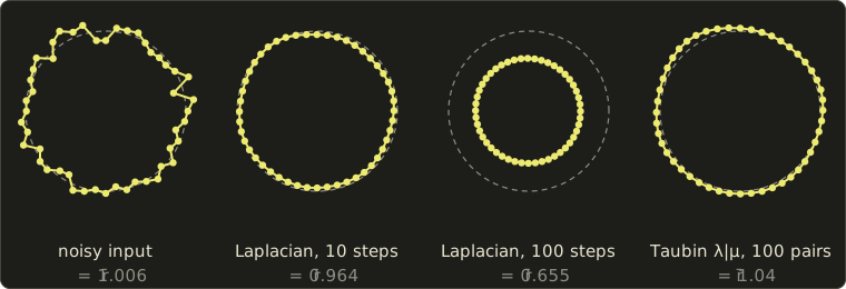
After 10 Laplacian steps the noise is gone, after 100 the curve has shrunk to two thirds, while 100 Taubin pairs keep the size (here it grows by about 3%, because is slightly above 1 for the lowest frequencies).
Real tools add variations: cotangent weights so vertices move only along the normal, implicit fairing (Desbrun et al., 1999), which solves a linear system for one big stable step, and feature-preserving filters (the mesh cousin of chapter 15's bilateral filter) that keep sharp edges.
A sculpting program's "smooth" brush is Laplacian smoothing inside the brush, and mesh tools offer Taubin smoothing for raw scans.
21.3 Mesh simplification with the quadric error metric
Chapter 9 introduced edge collapse (エッジ縮約): merge the two ends of an edge into one vertex, removing 1 vertex, 3 edges and 2 triangles.
It left open the real questions: which edge to collapse next, and where to put the new vertex.
The quadric error metric (二次誤差尺度, QEM) of Garland and Heckbert (1997) answers both, cheaply and well, and it's still the basis of most simplifiers.
The idea
Every vertex of the original mesh lies on the planes of its faces, and a good place for a new vertex is one that is still close to those planes.
So measure the error of a position as the sum of squared distances to a set of planes; give every vertex the planes of its faces, and when two vertices merge, let the new one inherit both sets.
In 2D, where the "planes" are lines, the error around a vertex looks like this:
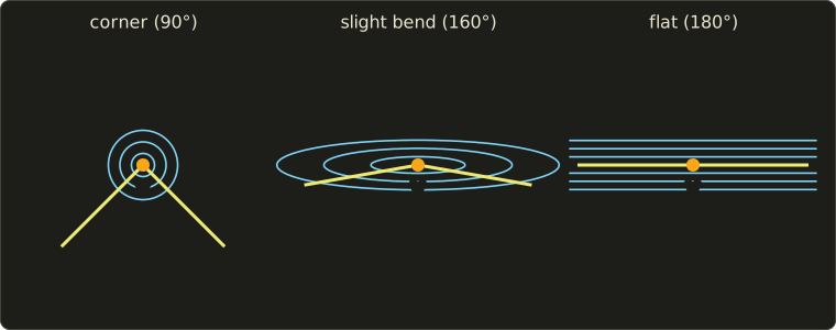
At a sharp corner the error grows quickly in every direction: the vertex is pinned.
At a slight bend it grows slowly along the curve: the vertex can slide.
On a flat part it's zero all along the line: removing the vertex costs nothing.
That's exactly what a simplifier should do: remove flat areas first, keep corners and creases.
Distance to a plane as a matrix product
Write a plane as with a unit normal , and collect its numbers in .
With the point in homogeneous coordinates, , the signed distance is a dot product (Linear Algebra chapter 4), and its square is a matrix "sandwich":
is a symmetric 4 × 4 matrix, the fundamental error quadric of the plane:
With several planes, the sum of squared distances is
So any number of planes is summarized by one symmetric 4 × 4 matrix , the vertex's quadric (二次誤差行列, クアドリック), 10 numbers in all, and merging two sets of planes is adding two matrices: .
Worked example: the quadric of a pyramid's apex
Take the square pyramid with apex and base corners .
The face through the apex, and is the plane ; with a unit normal, and
The other side faces are , and .
Adding all four, the mixed terms cancel in pairs ( has in one plane and in the opposite one, and so has ), and
The error is 0 at the apex and grows in every direction (an ellipsoid of constant error, the 3D version of the corner circles).
Moving the apex down to costs .
Check with one plane: the distance from to is , its square , and four planes give .
The best position for the new vertex
To collapse the edge from to , add their quadrics, , and find the position of smallest error.
Split into a 3 × 3 block , a column and a number ; then for a 3D point
This is a bowl-shaped quadratic, so its minimum is where the gradient vanishes:
a 3 × 3 linear system (Linear Algebra chapter 10), and substituting back gives the minimum error , the cost of the edge.
If is (nearly) singular there's no single best point: in a flat region, for example, every point of the plane has error 0.
Then implementations take the best of a few candidates, such as the two endpoints and the midpoint.
Worked example. Collapse the edge from the apex to the corner .
The corner touches the faces and and the base (unit normal , ):
The system reads
By symmetry , so the middle equation becomes ; the first gives ; substituting, , so and .
The optimum is , with error .
Collapsing onto the apex would cost 1, onto the corner 4, onto the midpoint 1.25.
The optimum beats them all and isn't even on the edge: QEM puts the vertex wherever the surface is approximated best.
(Collapsing a pyramid's apex is a bad idea for this tiny mesh, and the cost says so; an edge in a flat region costs exactly 0.)
The algorithm
- Compute a quadric for every vertex from the planes of its faces (often weighted by face area).
- For every edge, compute the optimal position and its cost from .
- Put all edges into a priority queue (a min-heap) ordered by cost.
- Collapse the cheapest edge to its optimal position, and give the new vertex .
- Recompute the costs of the edges around the new vertex, and repeat from step 4 until the target triangle count is reached.
Each collapse costs a few small matrix operations and a heap update, so the whole run takes about time for faces.
Real implementations check each collapse first: the two vertices of an interior edge must have exactly two common neighbors, or the result would be non-manifold (chapter 7); no neighboring triangle may flip over; open borders get a heavy extra plane through each border edge, perpendicular to its face, so the outline stays.
UVs, normals and colors can be added as extra dimensions of the quadric so that seams and color borders survive too (Garland and Heckbert, 1998; Hoppe, 1999).
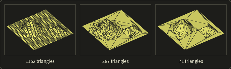
On this terrain, the flat ground is reduced to a few big triangles first, the small pyramid keeps its sharp edges, and the hill keeps its round shape with fewer, well-placed triangles.
In code: a quadric
Using linalg.hh from the Linear Algebra series, a quadric stores its 10 distinct numbers, is built from a triangle, adds, evaluates, and finds its optimum with Cramer's rule:
#include <cmath>
#include <cstdio>
#include "linalg.hh"

// A quadric Q = sum of q q^T for planes q = (a, b, c, d), stored as its 10 distinct entries.
struct Quadric {
  float a2 = 0, ab = 0, ac = 0, ad = 0, b2 = 0, bc = 0, bd = 0, c2 = 0, cd = 0, d2 = 0;

  // the plane through three points (unit normal n, d = -n.p)
  static Quadric fromTriangle(Vec3 p0, Vec3 p1, Vec3 p2) {
    Vec3 n = normalize(cross(p1 - p0, p2 - p0));
    float a = n.x, b = n.y, c = n.z, d = -dot(n, p0);
    return {a * a, a * b, a * c, a * d, b * b, b * c, b * d, c * c, c * d, d * d};
  }

  Quadric operator+(const Quadric &o) const {
    return {a2 + o.a2, ab + o.ab, ac + o.ac, ad + o.ad, b2 + o.b2,
            bc + o.bc, bd + o.bd, c2 + o.c2, cd + o.cd, d2 + o.d2};
  }

  // v^T Q v with v = (x, y, z, 1): the sum of squared distances to the planes
  float error(Vec3 p) const {
    float x = p.x, y = p.y, z = p.z;
    return a2 * x * x + 2 * ab * x * y + 2 * ac * x * z + 2 * ad * x
         + b2 * y * y + 2 * bc * y * z + 2 * bd * y
         + c2 * z * z + 2 * cd * z + d2;
  }

  // solve A v = -b by Cramer's rule; false if A is (nearly) singular
  bool optimum(Vec3 &v) const {
    float det = a2 * (b2 * c2 - bc * bc) - ab * (ab * c2 - bc * ac) + ac * (ab * bc - b2 * ac);
    if (std::fabs(det) < 1e-6f) return false;
    float rx = -ad, ry = -bd, rz = -cd;
    v.x = (rx * (b2 * c2 - bc * bc) - ab * (ry * c2 - bc * rz) + ac * (ry * bc - b2 * rz)) / det;
    v.y = (a2 * (ry * c2 - bc * rz) - rx * (ab * c2 - bc * ac) + ac * (ab * rz - ry * ac)) / det;
    v.z = (a2 * (b2 * rz - ry * bc) - ab * (ab * rz - ry * ac) + rx * (ab * bc - b2 * ac)) / det;
    return true;
  }
};

int main() {
  // the square pyramid of section 21.3: apex (0, 1, 0), base corners (+-1, 0, +-1)
  Vec3 apex = {0, 1, 0};
  Vec3 c0 = {1, 0, 1}, c1 = {1, 0, -1}, c2 = {-1, 0, -1}, c3 = {-1, 0, 1};
  Quadric qApex = Quadric::fromTriangle(apex, c0, c1) + Quadric::fromTriangle(apex, c1, c2)
                + Quadric::fromTriangle(apex, c2, c3) + Quadric::fromTriangle(apex, c3, c0);
  // the corner c0 touches two side faces and the base square
  Quadric qCorner = Quadric::fromTriangle(apex, c0, c1) + Quadric::fromTriangle(apex, c3, c0)
                  + Quadric::fromTriangle(c0, c3, c2);
  Quadric q = qApex + qCorner;

  printf("apex moved to (0, 0.5, 0): %.3f\n", qApex.error({0, 0.5f, 0}));
  printf("collapse to apex:     %.3f\n", q.error(apex));
  printf("collapse to corner:   %.3f\n", q.error(c0));
  printf("collapse to midpoint: %.3f\n", q.error(0.5f * (apex + c0)));
  Vec3 v;
  if (q.optimum(v)) printf("optimum (%.3f, %.3f, %.3f): %.3f\n", v.x, v.y, v.z, q.error(v));
  return 0;
}
apex moved to (0, 0.5, 0): 0.500
collapse to apex:     1.000
collapse to corner:   4.000
collapse to midpoint: 1.250
optimum (0.091, 0.727, 0.091): 0.727
Every number matches the hand calculation.
The sign of the normal doesn't matter: and give the same .
21.4 Progressive meshes and LOD streaming
Hoppe's progressive meshes
Run the simplifier all the way down and record every collapse.
Read backwards, each collapse is a vertex split (頂点分割): one vertex becomes two, and two triangles reappear.
That's the progressive mesh (プログレッシブメッシュ) of Hoppe (1996), a coarse base mesh followed by a list of vertex splits:
where each arrow is one vertex split and is the original mesh.
Every prefix of the list is a valid mesh, so one file holds every level of detail.
A 20,000-triangle model with a 200-triangle base mesh has splits, each adding 1 vertex and 2 triangles.
This gives continuous LOD (any number of splits, instead of chapter 9's few fixed versions), geomorphs (ジオモーフ, the new vertex slides out of its parent over a few frames, hiding popping), and progressive transmission (send first, then the splits, so the viewer sees a coarse model at once).
Hoppe's view-dependent refinement (1997) splits only where the model is near the camera, faces it, or forms the silhouette.
Choosing the level: screen-space error
The QEM cost gives a geometric error for each level (the square root of a sum of squared distances is a distance), and what matters is how big it looks on screen.
As in chapter 9, with a 60° vertical field of view on a 1080-pixel screen, one meter at distance covers
Worked example. A level whose largest error is 1 cm, seen from 10 m, is off by pixels: invisible.
From 5 m it's 1.87 pixels, so somewhere between 10 m and 5 m the renderer should switch to a finer level.
Engines pick, per object or region, the coarsest level whose screen-space error (スクリーン空間誤差) stays below about one pixel.
Streaming and cluster LODs
GPUs want big batches, not one vertex at a time, so modern engines build LODs from clusters: small groups of triangles, simplified with QEM and merged into a hierarchy, each drawn at its own level by its screen-space error.
Neighboring clusters at different levels must meet without cracks, so cluster borders are locked during one simplification step and freed in the next.
At the time of writing, Unreal Engine 5's Nanite is the best-known example: its documentation describes hierarchical clusters of triangles, swapped between levels of detail while rendering, joined without cracks, and streamed on demand so only visible detail is in memory.
It's still the progressive mesh idea, coarse first and refined where needed, with the cluster as the unit.
21.5 Remeshing and mesh repair
Isotropic remeshing
Scans and marching cubes give badly shaped triangles: slivers, mixed sizes, valences from 3 to 12.
Remeshing (リメッシュ) replaces them with new triangles on (almost) the same surface.
Isotropic remeshing (等方的リメッシュ) aims at nearly equilateral triangles of one target edge length ; the popular version of Botsch and Kobbelt (2004) repeats four steps about ten times:
- Split every edge longer than at its midpoint.
- Collapse every edge shorter than .
- Flip an edge (swap the diagonal of its two triangles) if that brings the valences of its four vertices closer to 6 (4 on a border).
- Relax: move each vertex towards its neighbors' centroid along the surface only (tangentially), then project it back onto the original.
Why ? With , an edge of is too long and its halves of are too short, so splitting only longer edges always helps.
For the flip, if the edge's two vertices have valence 7 and the two opposite vertices 5, the deviation from 6 is ; after the flip the edge's vertices lose a neighbor and the opposite ones gain one, giving and deviation 0, so we flip.
Step 4 is the umbrella operator with its normal part removed, so the surface doesn't shrink.
Repairing broken meshes
Meshes from scans, CAD exports and old games often break the rules of chapter 7.
Typical mesh repair (メッシュ修復) steps: weld vertices closer than a tolerance (turning a triangle soup back into a connected mesh), remove zero-area triangles, make the orientation consistent (walk across shared edges and flip any face whose winding disagrees with its neighbor), split non-manifold edges and vertices into separate manifold fans, fill holes (close each boundary loop with triangles, then smooth the patch to continue the surrounding surface), and remove self-intersections (hard; often done by computing an SDF and extracting a new surface, section 21.12).
Counting holes. The boundary edges are the half-edges without a twin, and following them gives the boundary loops.
The counts alone already tell you a lot: a connected orientable surface with genus (handles) and boundary loops has
A cube without its top face has , , , so , and : one hole.
Is it inside out? If the faces are consistently oriented but you don't know whether outwards or inwards, compute the signed volume (符号付き体積) with the divergence theorem:
Each term is six times the signed volume of the tetrahedron from the origin to the triangle.
For the tetrahedron , , , , the three faces through contribute 0, and the outward-wound face gives , so : positive, the normals point out.
A negative volume means the mesh is inside out and every face must be flipped.
21.6 Mesh parameterization
What a parameterization is
Texture mapping (chapter 11) needs a for every vertex, a map from the surface to the plane; computing it is mesh parameterization (パラメータ化), the algorithm behind UV unwrapping (UV展開).
Only a surface that is topologically a disc (one boundary loop, no handles) flattens in one piece, so meshes are first cut along seams (継ぎ目) into such charts, each chart is flattened, and the charts are packed into the texture atlas.
Measuring distortion
A curved surface can't be flattened without stretching, so the goal is small distortion.
On one triangle, the map from the triangle (in its own 2D frame) to UV space is affine, with a constant 2 × 2 Jacobian (ヤコビ行列).
Its singular values (特異値) are the largest and smallest stretch factors: a tiny circle on the surface becomes an ellipse with semi-axes and times its radius.
A map is conformal (等角) if (angles kept, sizes may change), authalic (等積) if (areas kept), and isometric (等長) if both are 1, which only surfaces that unroll flat (a cylinder, a cone) allow.
Worked example. A right triangle on the surface with legs 2 and 1 is mapped to the UV triangle , , .
The first leg shrinks by , the second keeps its length: , , .
: a checkerboard would show 1 × 2 rectangles on the surface instead of squares.
: this triangle gets half the texel density (テクセル密度, texels per square meter) of an undistorted one.
Tutte's embedding
Tutte (1963) proved that if you pin the boundary of a (3-connected planar) graph to a convex polygon and put every interior vertex at the average of its neighbors, no edges cross and every face is convex.
For a disc-shaped mesh: fix the boundary loop on a circle or a square, then solve
which is , the umbrella operator set to zero in UV space.
It's one sparse linear system, and it never produces flipped triangles, the most valuable guarantee a parameterization can have.
Floater showed that any positive weights that place each interior vertex at a convex combination of its neighbors keep the guarantee (1997), and his mean value weights (2003) follow the geometry far better than the plain average.
Worked example. A square chart has corners , , , and interior vertices , , with triangles , , , , , .
has the neighbors , and has :
Substituting into the first, , so and : inside the square, and no triangle flipped.
Notice that the 3D positions never appeared: the plain average uses only connectivity, so a mesh with very uneven triangles gets a badly distorted map.
Conformal maps: LSCM and ARAP
Least squares conformal maps (最小二乗等角写像, LSCM; Lévy, Petitjean, Ray and Maillot, 2002) aim at directly.
A map is conformal when on each triangle the direction is the direction turned by 90° with the same length (the Cauchy–Riemann equations).
That can't hold on every triangle at once, so LSCM minimizes the area-weighted squared violation; the energy is quadratic, so the minimum is again one sparse linear system, with two vertices pinned to fix position, rotation and scale, and a free boundary that finds its own natural shape.
It was designed for automatic texture atlases, and variants of it are behind the "unwrap" buttons of many tools.
ARAP parameterization (as-rigid-as-possible, Liu et al., 2008) asks each triangle's map to be as close as possible to a rotation (), alternating between the best rotation per triangle (local step) and one linear system for all UVs (global step).
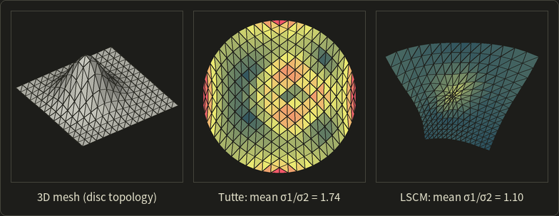
The colors show from 1 (dark teal) through 1.7 (yellow) to 3 and above (red).
Tutte squeezes the square border onto a circle and ignores the bump: angles are distorted almost everywhere (mean 1.74, worst at the four corners).
LSCM keeps the angles nearly right (mean 1.10) and lets the border bend instead; the bump's triangles shrink in UV space, the price of keeping angles.
Unwrapping tools then pack the charts with a few pixels of padding, so mipmaps don't bleed across.
21.7 Baking normal and displacement maps
Chapter 11 showed how a normal map makes a low-poly model look detailed, and said that normal maps are usually baked (ベイク) from a high-resolution sculpt; here is how.
The baking loop
The inputs are a low-poly mesh with good UVs (section 21.6) and a high-poly mesh of the same shape.
For every texel of the output map:
- Find the point on the low-poly surface that the texel covers, with its interpolated normal and tangent frame (chapter 11).
- Shoot a ray along from a start point outside, usually on a cage (ケージ), a copy of the low-poly mesh pushed outwards until it encloses the high-poly mesh, and find where it hits the high-poly mesh.
- Take the high-poly normal at the hit and convert it into tangent space: , which is multiplying by the transpose of the TBN matrix.
- Encode each component as and store it.
Worked example. On chapter 11's floor triangle, , , .
The ray from a texel hits the sculpt on a bump whose world-space normal is .
In tangent space: , encoded , which in 8 bits is .
That's exactly the texel chapter 11 decoded, and decoding gives back : baker and shader are inverses of each other.
A displacement map stores the signed distance along the normal instead.
If the bake maps heights from −0.05 to +0.05 to 0–1 and the sculpt is 0.03 above the low-poly surface, the stored value is , or 204 in 8 bits: a sample of a one-dimensional signed distance, the topic of the rest of this chapter.
Things that go wrong: a cage that is too tight starts rays inside the sculpt, one that is too loose hits the wrong part (an ear instead of the cheek); and if the baker and the renderer compute and differently, the lighting shows seams.
Many tools have standardized on MikkTSpace (Mikkelsen) for that reason; the glTF 2.0 specification, for example, says clients should compute missing tangents with MikkTSpace.
The same loop bakes ambient occlusion (many rays into the hemisphere at the hit), curvature, thickness or the sculpt's color.
21.8 Signed distance fields
Definition
Chapter 9 introduced the signed distance function (符号付き距離関数); stored on a grid or in a texture it's usually called a signed distance field (符号付き距離場), and both are abbreviated SDF.
For a solid with surface :
negative inside, as everywhere in this series.
Without the sign it's an unsigned distance field (符号無し距離場), which also works for open sheets and curves.
Properties
Three properties make SDFs special:
- The gradient has length 1 wherever it exists, : walking one unit straight away from the surface adds exactly one unit of distance. This is the eikonal equation (アイコナール方程式).
- The gradient is the normal: on the surface is the outward unit normal, and anywhere the closest surface point is .
- It's 1-Lipschitz: ; the value can't change faster than you move. This Lipschitz continuity (リプシッツ連続性) is what makes sphere tracing safe.
The gradient doesn't exist on the medial axis (中心軸), the points with two or more closest surface points, like a sphere's center or the diagonals inside a box; there the field has a ridge, but it lies away from the surface.
Worked example. For the unit sphere at : , of length 1, and the closest surface point is , which lies on the sphere.
Chapter 9's describes a sphere too, but isn't a distance (its gradient grows with the distance from the center), so none of these tricks work with it.
Exact SDFs and bounds
Sphere tracing doesn't need the exact distance.
A distance bound (距離の下界, conservative SDF) is any function with the right sign whose magnitude never exceeds the true distance, .
Every 1-Lipschitz function that is 0 exactly on the surface is one: a point at distance can't have a value above if the value changes at most 1 per unit.
Most "SDFs" in shaders are bounds, and that's fine; what breaks things is a function that overestimates.
Analytic SDFs
Simple shapes have exact formulas:
| Shape | SDF |
|---|---|
| sphere, center , radius | |
| plane, unit normal | |
| box, half sizes | with per component |
| torus in the xz plane, radii | |
| capsule from to , radius | distance to the segment minus |
In the box formula, folds the point into one octant (the box is symmetric) and measures how far each coordinate sticks out.
Outside, the positive parts of form the vector to the nearest face, edge or corner; inside, all parts are negative and the largest says how close the nearest face is.
With :
| outside part | inside part | nearest | |||
|---|---|---|---|---|---|
| 0 | 1 | face | |||
| 0 | 1.414 | edge | |||
| 0 | 1.732 | corner | |||
| 0 | −0.5 | face , from inside | |||
| 0 | −1 | center |
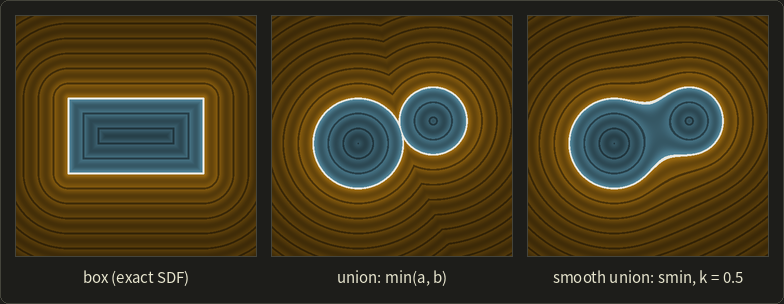
In the left picture (2D, orange outside, blue inside, a line every 0.2 units), the outside bands are rounded at the corners, where the distance is to a point; the inside bands have diagonal creases, the medial axis.
Transforming SDFs
To move or rotate a shape, transform the point with the inverse transform: rigid motions (chapter 5) keep distances, so is exact.
Uniform scaling by scales distances too: .
Non-uniform scaling doesn't preserve distances: is twice as long in x, but its values are no longer distances; multiplying by the smallest scale factor, , makes it a bound again.
21.9 Combining SDFs
Union, intersection and subtraction
Chapter 9's CSG operations
always give the right inside and outside.
Are the results distances?
The union is exact outside both shapes (the nearest surface really is the nearer of the two), but only a bound inside where they overlap; intersection and subtraction are exact inside, but only bounds outside.
All of them are 1-Lipschitz (min and max of 1-Lipschitz functions are), so all are safe for sphere tracing.
Worked example. Intersect the 2D half-planes and (, ), a quarter-plane with its corner at the origin.
At , , but the true distance to the corner is .
The bound is too small, which wastes a few steps near corners but never causes a miss.
The middle picture above shows the same effect: the union of two circles has a crease in its outside bands where the field switches from one circle to the other.
The smooth minimum
min makes a sharp crease where two shapes meet; organic modeling wants a fillet, like chapter 9's metaballs.
The smooth minimum (スムーズミン) blends near ; the common polynomial version with blend radius :
If , and the result is exactly ; if , it's exactly .
Only where does it blend, most at , where and the correction is .
Worked example with :
- : , . The blend pulls the surface 0.1 towards this point.
- , : , . Far from the seam nothing changes.
Is the result still safe for sphere tracing?
Differentiate, using and (from the definition of ):
and likewise .
So , a weighted average of two vectors of length at most 1, which has length at most 1: the smooth union of two SDFs is still 1-Lipschitz, a valid bound.
The exponential version has the same property, but changes the field everywhere a little (by at ).
The right picture above uses the polynomial version with : the circles are joined by a smooth neck, and the crease in the outside bands is gone.
Rounding, shells, repetition and displacement
- Rounding: grows the shape by and rounds its convex edges; a box with half sizes , minus , is a rounded box with half sizes .
- Shell: turns a solid into a hollow skin of thickness .
- Domain repetition: repeats a shape every units for the price of one. With , becomes , 0.5 left of its cell's center at 4.5. It's exact only if the shape fits well inside its cell; otherwise check the neighbor cells too.
- Displacement: adds bumps, but if changes faster than 1 per unit the result isn't 1-Lipschitz: has slope up to , so the sum changes up to per unit.
21.10 Sphere tracing
The algorithm and why it is safe
Sphere tracing (スフィアトレーシング) was described by Hart (1996) for rendering implicit surfaces; most people say ray marching (レイマーチング), although that name also covers fixed-step marching.
For a ray with unit :
until (hit) or exceeds a maximum (miss).
It can't jump through a surface because is a distance bound: the ball of radius around the current point contains no surface, so the next point, on that ball's boundary, can at most touch one.
Hart called these unbounding spheres.
The GLSL series, chapter 14 builds a complete sphere tracer step by step; here we look at how it behaves.
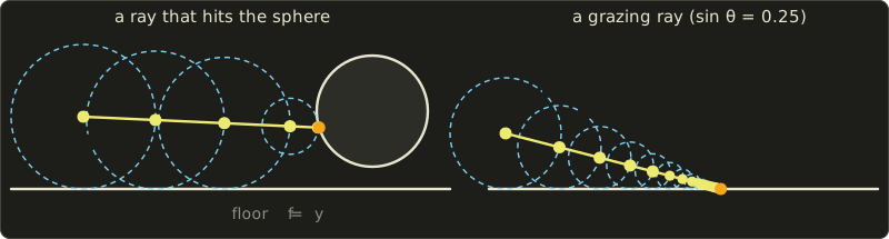
Worked step table for the left picture: the floor and a circle with center and radius 1, so ; the ray starts at with direction and stops when .
| Step | floor | circle | |||
|---|---|---|---|---|---|
| 0 | 0.000 | (0.000, 1.300) | 1.300 | 4.201 | 1.300 |
| 1 | 1.300 | (1.299, 1.240) | 1.240 | 2.905 | 1.240 |
| 2 | 2.540 | (2.538, 1.183) | 1.183 | 1.671 | 1.183 |
| 3 | 3.724 | (3.720, 1.129) | 1.129 | 0.505 | 0.505 |
| 4 | 4.229 | (4.224, 1.106) | 1.106 | 0.019 | 0.019 |
| 5 | 4.248 | (4.243, 1.105) | 1.105 | 0.001 | hit |
For three steps the floor is nearest and limits the steps; then the circle takes over, and two more steps reach it (the exact intersection is at ).
How fast it converges
Head-on, a ray reaches a plane in a single step, because the distance to the plane is exactly the distance along the ray.
At an angle it slows down: a ray at height above the plane , descending at angle (), loses of height per step, so the height is multiplied by each time:
With and :
| angle | factor per step | steps | |
|---|---|---|---|
| 1 | 90° | 0 | 1 |
| 0.5 | 30° | 0.5 | 10 |
| 0.1 | 5.7° | 0.9 | 66 |
| 0.01 | 0.57° | 0.99 | 688 |
For example , so 66 steps; the right picture shows , each circle 0.75 times the previous one.
Grazing rays along floors and past silhouettes are the expensive part of an SDF render, which is why tracers cap the step count and count "out of steps near a surface" as a hit.
Over-relaxation (過緩和, Keinert et al., 2014) steps by with around 1.2 to 1.6, and falls back to when the new unbounding sphere doesn't overlap the previous one (the step was too long).
Conversely, a function that is only -Lipschitz with (like the displaced shape above, ) must step by .
When to stop: the pixel footprint
A ray of one pixel is really a thin cone that widens with , so a fixed is too strict far away and too loose nearby.
With a 60° vertical field of view on a 1080-pixel screen, a pixel spans about radians, so at the cone is about wide.
Stopping when means "within a pixel": far surfaces stop early, near ones stay precise (Hart also used this cone to estimate anti-aliased coverage).
Normals from the gradient
The normal at the hit is the normalized gradient, estimated with central differences (中心差分) and a small :
Worked example. The unit sphere at with : and , so the x difference over is ; y gives 0.800 and z gives 0, the exact normal.
For an exact SDF the unnormalized estimate already has length close to 1, a handy debugging check.
Central differences need 6 evaluations; evaluating at the four corners of a tetrahedron, , , , , and using gives a vector proportional to the gradient with only 4.
Soft shadows and ambient occlusion
An SDF knows how close a ray passes to everything, which gives two famous cheap effects (both implemented in the GLSL series' chapter 14):
- Soft shadows: march towards the light; at each step (nearest distance over distance traveled) is roughly the angle by which the ray misses something, and , clamped to 1, estimates the visible part of the light. With , passing from an object after gives : 40% lit. Larger means a smaller light and harder shadows.
- Ambient occlusion: sample at a few distances along the normal; on an open surface , and any shortfall means something nearby blocks part of the sky.
Both are cheap approximations; chapter 24 covers real-time shadows and AO in general.
A sphere tracer in a shader
The core of an SDF renderer: a sphere, a smooth union, the scene and the march.
float sdSphere(float3 p, float r) { return length(p) - r; }

float smin(float a, float b, float k) {
  float h = saturate(0.5 + 0.5 * (b - a) / k);
  return lerp(b, a, h) - k * h * (1.0 - h);
}

// the scene: two spheres blended together, standing on the floor y = 0
float map(float3 p) {
  float blob = smin(sdSphere(p - float3(-0.8, 0.5, 0.0), 0.5),
                    sdSphere(p - float3(-0.2, 0.9, 0.1), 0.4), 0.3);
  return min(p.y, blob);
}

// sphere tracing; returns the distance along the ray, or -1.0 for a miss
float trace(float3 ro, float3 rd) {
  float t = 0.0;
  for (int i = 0; i < 128; i++) {
    float h = map(ro + t * rd);
    if (h < 0.001 * t) return t; // closer than about one pixel footprint
    t += h;
    if (t > 50.0) break;
  }
  return -1.0;
}
float sdSphere(vec3 p, float r) { return length(p) - r; }
float smin(float a, float b, float k) {
float h = clamp(0.5 + 0.5 * (b - a) / k, 0.0, 1.0);
return mix(b, a, h) - k * h * (1.0 - h);
}
// the scene: two spheres blended together, standing on the floor y = 0
float map(vec3 p) {
float blob = smin(sdSphere(p - vec3(-0.8, 0.5, 0.0), 0.5),
sdSphere(p - vec3(-0.2, 0.9, 0.1), 0.4), 0.3);
return min(p.y, blob);
}
// sphere tracing; returns the distance along the ray, or -1.0 for a miss
float trace(vec3 ro, vec3 rd) {
float t = 0.0;
for (int i = 0; i < 128; i++) {
float h = map(ro + t * rd);
if (h < 0.001 * t) return t; // closer than about one pixel footprint
t += h;
if (t > 50.0) break;
}
return -1.0;
}float sdSphere(float3 p, float r) { return length(p) - r; }
float smin(float a, float b, float k) {
float h = saturate(0.5 + 0.5 * (b - a) / k);
return lerp(b, a, h) - k * h * (1.0 - h);
}
// the scene: two spheres blended together, standing on the floor y = 0
float map(float3 p) {
float blob = smin(sdSphere(p - float3(-0.8, 0.5, 0.0), 0.5),
sdSphere(p - float3(-0.2, 0.9, 0.1), 0.4), 0.3);
return min(p.y, blob);
}
// sphere tracing; returns the distance along the ray, or -1.0 for a miss
float trace(float3 ro, float3 rd) {
float t = 0.0;
for (int i = 0; i < 128; i++) {
float h = map(ro + t * rd);
if (h < 0.001 * t) return t; // closer than about one pixel footprint
t += h;
if (t > 50.0) break;
}
return -1.0;
}The picture below was rendered on the CPU with the techniques of this chapter: a rounded box smoothly blended with a sphere, a torus, an endless row of pillars by domain repetition, a checkered floor, soft shadows with , five-sample ambient occlusion, tetrahedral normals and a little fog.
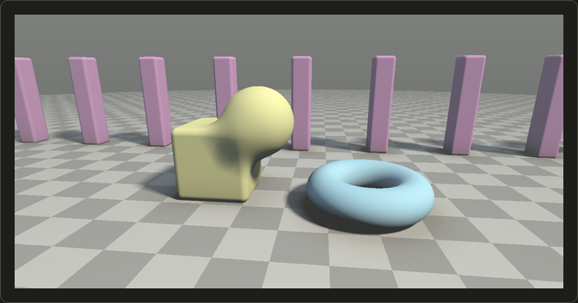
Not a single triangle was involved.
21.11 SDFs from meshes and SDF grids
Distance to a triangle mesh
To use SDF techniques on ordinary models we need the SDF of a mesh: the unsigned distance is the minimum over all triangles of the point-to-triangle distance (project onto the triangle's plane, then check whether the nearest point is inside, on an edge or at a corner), with a bounding volume hierarchy (chapter 12) to skip far triangles.
The hard part is the sign:
- Ray parity: count the surface crossings of a ray from the point; odd means inside. Rays that graze an edge or a vertex miscount, so implementations vote with several rays.
- Angle-weighted pseudonormals (擬法線, Bærentzen and Aanæs, 2005): if the vector from the closest surface point to the query point points against the normal there, the point is inside. When the closest point is on an edge or a vertex, the angle-weighted average of the face normals (chapter 9) makes the test correct for closed meshes.
- Generalized winding numbers (一般化回転数, Jacobson, Kavan and Sorkine-Hornung, 2013): sum the signed solid angles of all triangles seen from the point and divide by : 1 inside and 0 outside a closed mesh, a fraction near holes, where thresholding at 0.5 still gives a sensible answer.
Worked example. From the center of a cube, each face covers of the full sphere of directions, so the winding number is : inside.
Delete one face: ray parity now depends on the ray's direction, but the winding number is , still inside, as a human would say.
Storing SDFs on grids
A general shape's SDF has no formula, so it's sampled on a 3D grid and read with trilinear interpolation (3線型補間, the 3D version of chapter 11's bilinear filtering).
Dense grids are large: samples at 2 bytes take bytes, 32 MiB, for one object.
But mostly only values near the surface matter, so engines keep a narrow band (ナローバンド, only samples with small ) or a sparse grid (疎な格子): small bricks of voxels, allocated only near the surface and found through a tree or a hash.
OpenVDB (Museth, 2013), widely used in film effects, is such a hierarchical sparse grid.
Worked example. A sphere of radius 100 voxels in a grid with a band of voxels: the band is the shell between radii 97 and 103, voxels, about 4.5% of the grid's .
A surface is two-dimensional, so the band grows with the square of the resolution, not the cube.
Grid SDFs come from the closest-triangle search above, or from distance transforms that propagate distances outwards from the surface (fast marching, fast sweeping, or jump flooding on GPUs).
In practice
At the time of writing, Unreal Engine is a well-known example: its documentation says that Lumen's software ray tracing traces each mesh's own distance field for the first two meters of a ray and a merged global distance field for the rest, and the engine also uses mesh distance fields for soft shadows and ambient occlusion.
Physics engines use SDFs for collisions (penetration depth and push-out direction are just and , see chapter 26), and film tools use sparse level sets for liquids, smoke and fracture.
Fonts and decals: SDF textures
A glyph or decal stored as an alpha mask gets blurry or blobby when magnified, because filtering coverage values doesn't know where the edge is.
Green (Valve, 2007) proposed storing a distance field instead: compute it from a high-resolution binary image (his typical example: 4096 × 4096 down to 64 × 64), store it in one channel of a small texture, and draw it with a plain alpha test (アルファテスト) at 0.5.
Bilinear interpolation of distances is nearly linear near the edge, so the 0.5 contour stays sharp at large magnifications; Valve used it in Team Fortress 2, for example for decals.
An 8-bit channel holds a limited range, so a spread (in texels) maps it to 0–1; with this series' sign convention, so that inside is above 0.5:
Worked example. With texels: on the edge (128 in 8 bits); 2 texels inside, (191); 4 or more texels outside, .
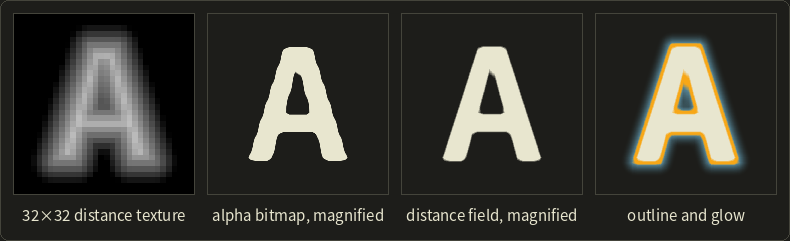
Both magnified letters come from 32 × 32 textures: the alpha bitmap's edges wobble, the distance field's stay straight.
Effects are just other thresholds: an outline is a band between two values, a glow a soft ramp further out.
In the shader, the edge is anti-aliased over one screen pixel, whose size in texture values the derivative fwidth provides:
// v: the distance texture's value at this pixel (0.5 on the edge, larger inside)
float sdfCoverage(float v) {
  float w = 0.5 * fwidth(v); // half a screen pixel, in texture value units
  return smoothstep(0.5 - w, 0.5 + w, v);
}
// v: the distance texture's value at this pixel (0.5 on the edge, larger inside)
float sdfCoverage(float v) {
float w = 0.5 * fwidth(v); // half a screen pixel, in texture value units
return smoothstep(0.5 - w, 0.5 + w, v);
}// v: the distance texture's value at this pixel (0.5 on the edge, larger inside)
float sdfCoverage(float v) {
float w = 0.5 * fwidth(v); // half a screen pixel, in texture value units
return smoothstep(0.5 - w, 0.5 + w, v);
}
The weakness shows at the apex of the "A": sharp corners get slightly rounded, because one distance can't represent two edges meeting at an angle.
Multi-channel SDFs (MSDF, Chlumský and colleagues, with the msdfgen tool) store three distances in RGB and take their median, which keeps corners sharp.
You'll render text in the OpenGL series, chapter 26, which mentions SDF atlases as the way engines keep text sharp at any size.
21.12 From SDFs back to meshes
To 3D print a sculpt, simulate it or rasterize it, an SDF often has to become a mesh again.
Chapter 9's marching cubes puts a vertex on every grid edge with a sign change and connects them by a 256-case table; since every vertex lies on a grid edge, sharp features inside a cell, like a box corner, are cut off.
Two dual methods put the vertices inside the cells instead:
- Surface nets (サーフェスネット, Gibson, 1998): one vertex in every cell the surface passes through, at the average of the cell's edge crossings; across every grid edge with a sign change, connect the vertices of the cells around it (four cells and a quad in 3D, two cells and a segment in 2D). No case table and better shaped faces, but corners are still rounded.
- Dual contouring (デュアルコンタリング, Ju, Losasso, Schaefer and Warren, 2002): the same connectivity, but each vertex also uses the normals at the crossings (from ; crossings plus normals are called Hermite data, エルミートデータ). Each crossing with normal defines a plane, and the vertex minimizes .
That's a sum of squared distances to planes, exactly the quadric of section 21.3; the paper calls it a QEF (quadratic error function) and solves with the same way.
Worked example (2D). The cell contains the corner of a shape bounded by and (inside: and ).
The bottom edge is crossed at with normal , the left edge at with normal .
Marching squares joins the crossings with a segment from to , cutting the corner off; surface nets puts the vertex at their average ; dual contouring minimizes , whose minimum is the corner itself.
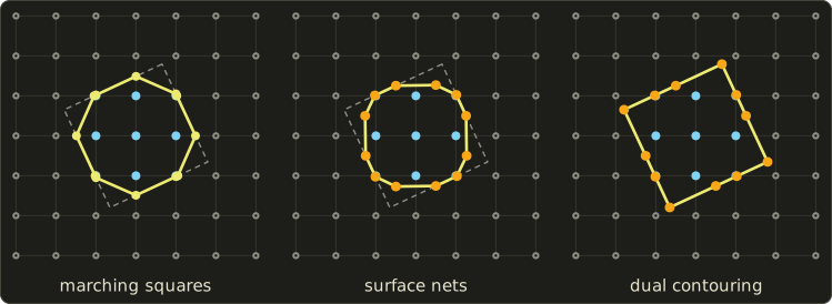
Marching squares turns the square into an octagon, surface nets into a rounded square, dual contouring recovers all four corners.
The price: a QEF vertex can land outside its cell or make the surface self-intersect, so implementations clamp it and take care to keep the result manifold.
Voxel terrains and SDF sculpting tools often use these dual methods.
Exam points
This chapter goes beyond the syllabus, but these Part 1 points are worth being sure about:
- Polygon surfaces (chapter 9): an edge collapse removes 1 vertex, 3 edges and 2 triangles; its inverse is a vertex split; recorded collapses form a progressive mesh; popping is the visible jump between LOD levels.
- Euler's formula (chapter 7): for a closed surface without holes, so its total angle defect is .
- Implicit surfaces (chapter 9): CSG by min and max; an SDF's value is the distance to the surface; marching cubes places vertices on grid edges by linear interpolation.
- Texture mapping (chapter 11): UV unwrapping cuts the surface along seams; normal maps are baked from a high-polygon model and stored in tangent space.
21.13 Summary
- Meshes get a Laplacian (the umbrella operator , or cotangent weights) and a Gaussian curvature (the angle defect , in total ).
- Laplacian smoothing is a leaky low-pass filter that shrinks the shape; Taubin's steps pass frequencies below .
- QEM sums a vertex's plane quadrics into one 4 × 4 matrix; an edge costs the minimum of , at ; cheapest first, so flat regions vanish and corners stay.
- Progressive meshes give continuous LOD, geomorphs and streaming; engines refine clusters by screen-space error.
- Remeshing splits, collapses, flips and relaxes; repair welds, reorients and fills holes, helped by Euler counts and the signed volume.
- Parameterization flattens disc-like charts, with distortion measured by the Jacobian's singular values; Tutte never flips triangles, LSCM keeps angles, ARAP aims at rigid triangles.
- Baking casts rays from a cage to the high-poly mesh; baker and renderer must agree on the tangent frame.
- An SDF's gradient is the unit normal and the field is 1-Lipschitz; any 1-Lipschitz bound with the right sign is safe for sphere tracing, and min, max and the polynomial smin keep that.
- Sphere tracing can't miss a surface but is slow at grazing angles; normals, soft shadows and AO come almost for free.
- Mesh SDFs need a robust sign (pseudonormals, winding numbers) and narrow-band or sparse grids; SDF textures keep text sharp.
- Surface nets and dual contouring put vertices inside cells; dual contouring's QEF is the QEM quadric again and keeps corners.
21.14 Key terms
| English | 日本語 |
|---|---|
| discrete differential geometry | 離散微分幾何 |
| one-ring | 1-リング近傍 |
| umbrella operator | アンブレラ演算子 |
| cotangent weights | コタンジェント重み |
| mean curvature, Gaussian curvature | 平均曲率、ガウス曲率 |
| angle defect | 角度欠損 |
| Gauss–Bonnet theorem | ガウス・ボネの定理 |
| smoothing, fairing | 平滑化、フェアリング |
| Laplacian smoothing | ラプラシアンスムージング |
| low-pass filter | ローパスフィルタ |
| pass-band frequency | 通過帯域周波数 |
| quadric error metric (QEM) | 二次誤差尺度(QEM) |
| quadric | 二次誤差行列(クアドリック) |
| edge collapse, vertex split | エッジ縮約、頂点分割 |
| progressive mesh | プログレッシブメッシュ |
| geomorph | ジオモーフ |
| screen-space error | スクリーン空間誤差 |
| isotropic remeshing | 等方的リメッシュ |
| mesh repair | メッシュ修復 |
| signed volume | 符号付き体積 |
| mesh parameterization | メッシュのパラメータ化 |
| Jacobian, singular value | ヤコビ行列、特異値 |
| conformal, authalic, isometric | 等角、等積、等長 |
| texel density | テクセル密度 |
| Tutte embedding | Tutteの埋め込み |
| least squares conformal maps (LSCM) | 最小二乗等角写像(LSCM) |
| baking, cage | ベイク、ケージ |
| signed distance field (SDF) | 符号付き距離場(SDF) |
| unsigned distance field | 符号無し距離場 |
| eikonal equation | アイコナール方程式 |
| Lipschitz continuity | リプシッツ連続性 |
| medial axis | 中心軸 |
| distance bound | 距離の下界 |
| smooth minimum | スムーズミン |
| sphere tracing, ray marching | スフィアトレーシング、レイマーチング |
| over-relaxation | 過緩和 |
| central differences | 中心差分 |
| pseudonormal | 擬法線 |
| generalized winding number | 一般化回転数 |
| narrow band, sparse grid | ナローバンド、疎な格子 |
| trilinear interpolation | 3線型補間(トライリニア補間) |
| alpha test | アルファテスト |
| surface nets | サーフェスネット |
| dual contouring | デュアルコンタリング |
| Hermite data | エルミートデータ |
21.15 Challenges
- ★ Compute the angle defect at a vertex of a regular icosahedron (five equilateral triangles at each of its 12 vertices) and the total over all vertices, and compare with . Then compute the defect where seven equilateral triangles meet. What kind of point is that?
- ★ For the box with half sizes , compute the SDF at , , and , and name the nearest feature (face, edge or corner) for each. Then compute, at , the SDF of the rounded box with rounding radius 0.2 and the same outer size.
- ★★ A vertex has the planes , and (one face each); write its quadric . A second vertex has the single plane . Build , solve , give the collapse cost, and explain the result in words.
- ★★ For Taubin smoothing with and , compute and the factor of one pair for , and . Which of these frequencies are kept, damped or removed?
- ★★★ Show that the exponential smooth minimum is 1-Lipschitz when and are, and that it lies between and . Then explain why a sphere tracer must take smaller steps for , and by at most what factor.
Multiple choice
Q1 ★ Which of the following correctly describes mesh simplification with the quadric error metric (QEM)?
| A | Each vertex stores a symmetric 4 × 4 matrix, the sum of q qᵀ over the planes of its faces; the cost of collapsing an edge is the error of the new position under the sum of the two matrices, and that sum becomes the new vertex's matrix. |
| B | After every collapse, the algorithm computes the exact Hausdorff distance between the original and the simplified mesh and uses it as the cost. |
| C | Edges are always collapsed in order of their length, shortest first, regardless of the shape. |
| D | The new vertex is always placed at the midpoint of the collapsed edge, because the quadric cannot be minimized in closed form. |
| E | A vertex in a perfectly flat region has a very large error, so flat regions are kept and curved regions are simplified first. |
Q2 ★ Which of the following statements about signed distance fields (SDFs) and sphere tracing is correct?
| A | Sphere tracing needs the exact distance; a function that underestimates the distance makes rays pass through surfaces. |
| B | The minimum of two exact SDFs is again an exact SDF everywhere, both inside and outside the union. |
| C | The gradient of an exact SDF has length 0 on the surface, which is why normals must be computed by finite differences. |
| D | If the function is 1-Lipschitz with the right sign, stepping along the ray by its value can never jump over the surface, but rays at grazing angles need many steps. |
| E | Stretching a shape by evaluating f(x/2, y, z) gives the exact SDF of the stretched shape. |
Q3 ★★ Using the polynomial smooth minimum smin(a, b) = (1 − h) b + h a − k h (1 − h), with h = clamp(0.5 + (b − a) / (2k), 0, 1), what is smin(0.3, 0.1) for k = 0.4?
| A | 0.1 |
| B | 0.075 |
| C | 0.15 |
| D | 0 |
| E | 0.2 |
21.16 Practical assignment
On graph paper, build a small 2D SDF scene, sphere trace it with a compass, then smooth and simplify its outline as a mesh.
You need graph paper (at least 50 × 30 squares), a ruler, a compass, a pencil, two colored pens and a calculator.
Use 1 unit = 4 squares, with from −5 to 7 to the right and from −2 to 4 upwards.
The scene is a box with center and half sizes and a circle with center and radius 1:
- The field. Draw both shapes. Compute at , , , , and , write each value next to its point, and mark the points inside. For and , draw the shortest segment to the surface and measure it.
- Three rays. Sphere trace ray A from in direction and ray B from in direction : at each point compute , and , draw the empty circle with the compass, and step to its edge along the ray; stop when . Keep a table of , the point and the distances (three decimals). Then trace ray C from in direction , which passes just above the circle, until , and mark where its steps are shortest.
- A normal. At ray B's hit point, estimate the normal by central differences with , normalize it, and compare it with the circle's exact normal .
- Smooth union. With , compute at and and compare with . Sketch with the second pen how the smooth union changes the outline between the shapes.
- Smoothing the outline. Treat the box outline as a closed mesh of 8 noisy vertices, in this order: , , , , , , , . Compute its area with the shoelace formula . Apply one umbrella step with (each vertex towards the midpoint of its two neighbors), draw it and compute the area; then apply one step with to the result, draw it and compute the area again.
- Simplifying the outline. Take the clean outline with 8 vertices at the box's corners and edge midpoints. With 2D quadrics of lines (, ), compute the cost of collapsing the midpoint onto the corner and the cost of collapsing the corner onto the midpoint. Which would QEM choose, and what remains after collapsing all four midpoints?
How to check yourself: each step lands on the previous circle, and no circle crosses an outline (they may touch it); rays A and B end with near the box's top and the circle's upper right, while ray C escapes, with its shortest steps just above the circle; your normal has length close to 1 and matches the exact one to about two decimals; at both points, with equality where the distances differ by at least ; the step shrinks the area and the step brings it back close to the original; the midpoint collapses cost 0 and the corner collapses don't, so QEM ends with the four corners.
コメント(0)
まだコメントはありません。
ログインするとコメント出来ます。