17. CG Systems
Every chapter so far was about algorithms; this one is about the machines and programs that run them: the processors that run the pipeline, the software people work with, the devices that bring shapes into the computer and pictures out of it, and the media that store the results.
Many design decisions in graphics only make sense once you know the hardware: why games count milliseconds, why the GPU wants thousands of identical small jobs, why a 3D scanner fails on a glass vase, why a 3D printer refuses a mesh with a hole.
For the exam, this chapter covers syllabus area 8, CG systems (CGシステム), with its items CG software (CG用ソフトウェア), real-time 3D CG systems (リアルタイム3次元CGシステム), 3D data input devices (3次元データ入力装置), 3D data output devices (3次元データ出力装置) and recording media (記録メディア).
It builds on the camera and compression of chapter 2, color and depth cues from chapter 3, the GPU pipeline of chapter 6, solids and meshes from chapter 7 and chapter 9, and the rendering of chapters 10 to 12.
Hardware changes fast.
Read every capacity, speed and product generation in this chapter as "at the time of writing" (late 2026); the principles behind them change much more slowly, and they are what's worth knowing for the exam.
Product and tool names appear only as examples, not as recommendations.
17.1 What a CG system is
A CG system (CGシステム) is everything needed to make computer graphics: hardware, software, and the procedures that connect them.
From a phone to a film studio, it has the same four parts:
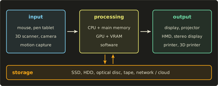
- Input (入力): mouse and pen tablet, cameras and 3D scanners, motion capture.
- Processing (処理): CPU and main memory, GPU and its memory, and the software running on them.
- Output (出力): displays, projectors, head-mounted displays, printers and 3D printers.
- Storage (記録): SSDs, hard disks, optical discs, tape, network and cloud storage.
A workstation (ワークステーション), once a special, expensive computer for CAD and CG, is today usually a powerful PC with a professional GPU and lots of memory.
The rest of the chapter follows the picture: processing (17.2 to 17.4), input (17.5), output (17.6 and 17.7) and storage (17.8).
17.2 CPU, GPU and memory
Two kinds of processor
The CPU runs the operating system, the application logic, physics, animation and file loading.
The GPU runs the drawing pipeline of chapter 6 (section 6.5).
Both compute with numbers, but they are built for opposite goals:
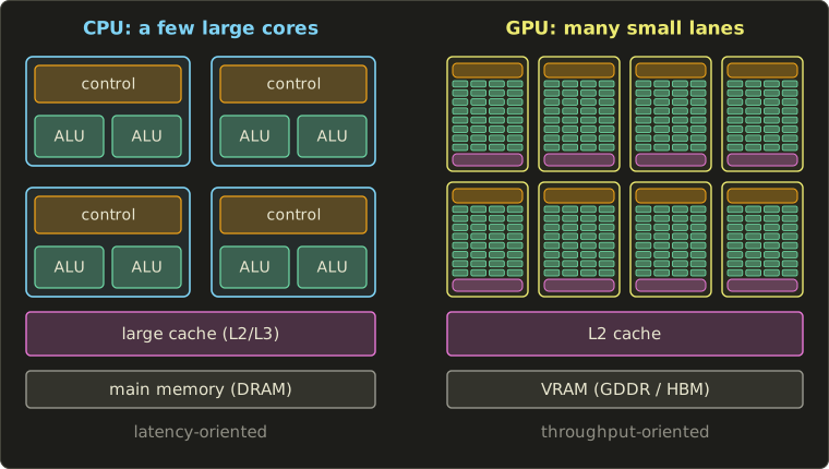
- A CPU has a few large cores (a handful to a few dozen). Much of each core is control logic (orange): branch prediction, out-of-order execution, plus large caches (pink). It is built for low latency (レイテンシ): finish one complicated, branchy task as soon as possible.
- A GPU has many small lanes (green), grouped into blocks called streaming multiprocessors (SM) or compute units (CU) depending on the vendor; a high-end desktop GPU at the time of writing has over 20,000 lanes. Each block shares one control unit. It is built for throughput (スループット): finish millions of similar small tasks per frame, even if each one waits a while.
Graphics is the perfect job for the second design.
A 1920 × 1080 frame has 2,073,600 pixels, and the fragment shader runs the same program on every one of them with different inputs; the same holds for vertices, rays and particles.
This is data parallelism (データ並列): the same operation on many data items at once.
SIMT and branch divergence
A GPU block runs its lanes in lock-step groups, typically of 32 (some vendors use 32 or 64), called a warp or wavefront.
All lanes of the group execute the same instruction at the same time, each on its own data: SIMT (single instruction, multiple threads).
To the programmer each lane looks like an independent thread; underneath, 32 of them share one instruction stream.
The consequence is branch divergence (分岐ダイバージェンス): if some lanes of a group take the if branch and others the else branch, the group runs both branches one after the other, with the lanes that didn't take a branch switched off.
Worked example. Path A costs 100 cycles, path B costs 50.
In a group of 32 lanes, 10 take A and 22 take B.
- Uniform groups would need 100 cycles (all A) or 50 cycles (all B).
- This divergent group needs cycles.
- Useful work: lane-cycles out of , an efficiency of .
That's why shader programmers prefer branches that are the same for neighboring pixels ("is this material metal?") over branches that change from pixel to pixel.
GPUs hide the other big cost, waiting for memory, with sheer numbers: while one group waits hundreds of cycles for a texture value, the block switches to another group that is ready.
The same lanes also run compute shaders (GPGPU) for physics, image processing and machine learning; the GLSL series, chapter 15 shows one.
Memory and bandwidth
The GPU has its own fast memory, VRAM (ビデオメモリ): GDDR chips on the board, or HBM stacked next to the chip on some high-end and data-center GPUs; consumer cards at the time of writing carry roughly 8 to 32 GB.
It holds the frame buffer, depth buffer, textures, vertex and index buffers and ray-tracing acceleration structures.
Integrated GPUs (laptops, phones, game consoles) instead share one unified memory with the CPU, which saves copying but shares the bandwidth.
For real-time graphics, the bandwidth (帯域幅) of the memory matters as much as its size.
A high-end card at the time of writing has a 512-bit memory bus at 28 Gbit/s per pin: GB/s, about 1.8 TB/s.
Worked example: frame-buffer traffic at 4K and 60 Hz.
A 4K UHD frame has pixels; at 4 bytes per pixel that's bytes, about 33.2 MB, and writing it 60 times a second costs about 1.99 GB/s.
Real rendering touches each pixel several times.
Assume each pixel is covered by 3 surfaces (overdraw 3), and each time the depth test reads 4 bytes of depth, writes 4 bytes of depth and writes 4 bytes of color; then the display reads the color once:
That's only about 1.1 % of 1792 GB/s.
The frame buffer itself is cheap; the bandwidth goes to textures (a single 4096 × 4096 RGBA8 texture with mipmaps is MB, see chapter 11), G-buffers and post-processing (section 17.4) and shadow maps.
On-chip caches avoid fetching the same data twice for neighboring pixels, and data needed every frame should stay in VRAM, because the bus from the CPU (PCI Express in PCs) is far slower.
Render farms and the studio pipeline
Offline rendering for film (chapter 12) can take minutes to hours per frame.
A render farm (レンダーファーム) is a cluster of computers (render nodes) that render different frames at the same time, fed by a job scheduler.
Frames are independent, so the speed-up is almost perfect.
Worked example. A 90-minute film at 24 frames per second has frames.
At 2 hours per frame that's node-hours, almost 30 years on one machine; on 1,000 nodes, hours, about 10.8 days.
Cloud rendering (クラウドレンダリング) rents such nodes by the hour, so a small studio can use a thousand machines for a week without owning them.
In a studio, data flows between departments (modeling → rigging → animation → lighting → rendering → compositing), and two tools keep it under control:
- Asset management (アセット管理): every model, texture, rig and shot is an asset with versions, an owner and dependencies, tracked in a database so tools can find "the approved version".
- Version control (バージョン管理): every change is recorded and can be compared or undone; large binary assets need systems that handle huge files and locking.
Exam points
- CPU: few complex cores, low latency, large caches. GPU: many simple lanes, high throughput, data parallel (SIMT).
- Divergent branches in a warp run both paths; memory latency is hidden by switching between many threads.
- VRAM bandwidth limits real-time rendering; integrated GPUs share memory with the CPU.
- Render farms parallelize by frame; cloud rendering rents the nodes.
17.3 CG software
Categories
CG software (CG用ソフトウェア) comes in a few families.
The names in the table are well-known examples in no particular order, not recommendations; most studios combine several.
| Category | What it does | Examples |
|---|---|---|
| DCC tools (modeling, animation) | polygon and subdivision modeling, UVs, rigging, keyframe animation, rendering | Blender, Maya, 3ds Max |
| Procedural tools | node networks that generate geometry, effects and simulations (chapter 9) | Houdini, Blender's Geometry Nodes |
| Digital sculpting | shaping millions of polygons like clay, then baking normal maps (chapter 11) | ZBrush, Blender's sculpt mode |
| CAD | precise solids for manufacturing: B-rep, NURBS, features (chapters 7 and 8) | AutoCAD, SolidWorks, FreeCAD |
| Renderers | offline path tracing for film (chapter 12) | RenderMan, Arnold, V-Ray, Cycles |
| Compositing | layering rendered passes and live action (chapter 14) | Nuke, After Effects |
| Image editing and painting | retouching, painting textures (chapter 15) | Photoshop, GIMP, Krita, Substance Painter |
| Game engines | real-time rendering plus physics, audio, scripting and an editor | Unreal Engine, Unity, Godot |
DCC stands for digital content creation (デジタルコンテンツ制作): the general tools artists build assets with.
A game engine (ゲームエンジン) is a renderer and a framework at once: you write the game logic against it, and it runs the frame loop of section 17.4.
Interchange formats
Because studios combine tools, files must move between them.
Chapter 9 (section 9.1) introduced OBJ, PLY, STL and glTF; here is the bigger picture:
| Format | Stores | Typical use |
|---|---|---|
| OBJ | polygons, UVs, normals; materials in .mtl |
simple exchange of static meshes |
| FBX | meshes, materials, skeletons, skinning, animation; proprietary (Autodesk) | animated characters between DCC tools and engines |
| glTF 2.0 | meshes, PBR materials, hierarchy, skins, animation; open Khronos and ISO standard | delivery to real-time engines and the web |
| USD | whole scenes as layers that override each other; open source (Pixar, 2016) | film and VFX pipelines, many departments on one scene |
| Alembic | baked geometry caches: the vertex positions of every frame | handing simulations and deformed meshes to lighting |
| STL, 3MF | closed triangle meshes for manufacturing (section 17.7) | 3D printing |
| OpenEXR | floating-point HDR images with many channels | rendered passes, textures |
The difference between FBX/glTF and Alembic is worth knowing: the first two store a rig and its animated joint values, so the receiving program must compute the deformation itself; Alembic stores the result, every vertex of every frame, which is bigger but looks the same everywhere.
Almost every DCC tool can be extended: scripting (スクリプト), usually in Python, automates repetitive work and much of a studio's pipeline, and plug-ins (プラグイン), usually in C++ against the tool's SDK, add deformers, shaders, file formats or whole renderers.
Graphics APIs and shading languages
Programs talk to the GPU through a graphics API (グラフィックスAPI) and its driver:
| API | Platforms | Notes |
|---|---|---|
| OpenGL (OpenGL ES, WebGL) | desktop, mobile, web | older and high level, the driver does much implicitly; the OpenGL series teaches it |
| Vulkan | Windows, Linux, Android and others | low-level and explicit: the application manages memory, synchronization and command buffers |
| Direct3D 12 | Windows, Xbox | low-level, similar in spirit to Vulkan |
| Metal | Apple platforms | low-level, Apple's own |
| WebGPU | web browsers | a modern explicit API for the web |
Explicit APIs give the programmer more work but less hidden driver overhead and better use of many CPU cores.
Shaders are written in a shading language (シェーディング言語): GLSL (OpenGL, Vulkan), HLSL (Direct3D, also Vulkan), MSL (Metal), WGSL (WebGPU), and Slang, which compiles to several of them and has been hosted by the Khronos Group since 2024.
Vulkan consumes shaders as SPIR-V, an intermediate binary form, so any language with a SPIR-V compiler works.
You'll write shaders yourself in the GLSL series; the samples in this series show Slang, GLSL and HLSL side by side.
Middleware (ミドルウェア) solves one problem well between the application and the platform: physics, audio, animation, UI, video playback; a game engine is, in a sense, a bundle of middleware with an editor on top.
17.4 Real-time 3D CG systems
A real-time 3D CG system (リアルタイム3次元CGシステム) produces each image fast enough for interaction: games, simulators, VR, CAD viewports.
Its heart is the GPU pipeline of chapter 6; here we look at the hardware behind it and the timing around it.
Inside a GPU
Early GPUs had separate hardware for vertex and pixel shaders, and one of them often sat idle.
Since the mid-2000s GPUs use a unified shader architecture (ユニファイドシェーダーアーキテクチャ): the same programmable lanes run vertex, fragment and compute shaders, whatever the workload needs.
Around them sit fixed-function units for jobs so common that dedicated hardware does them faster and with less power:
- the rasterizer (ラスタライザ), which turns triangles into fragments (chapter 6, section 6.9);
- texture units, which compute texel addresses and filter (chapter 11);
- ROPs (render output units), which do the depth and stencil tests, blending and the frame-buffer writes;
- caches and memory controllers, the video encoder/decoder and the display controller;
- on recent GPUs, ray tracing units for BVH traversal and ray–triangle tests (chapter 12, section 12.9) and matrix units for neural networks such as AI upscalers and denoisers.
Frame rate and frame time
Real-time rendering is measured in frames per second (fps, フレームレート) or, more usefully, in milliseconds per frame (フレームタイム).
They are reciprocals: 30 fps is 33.3 ms, 60 fps is 16.7 ms, 120 fps is 8.33 ms.
Milliseconds are the engineering unit because costs add up: going from 30 to 60 fps means cutting 16.7 ms of work, going from 120 to 240 fps only ms, although both "double the frame rate".
How a game loop divides this frame budget is the subject of chapter 14.
Tearing, v-sync and buffering
Chapter 6 (section 6.5) explained double buffering, tearing (テアリング) and v-sync (垂直同期); let's see them on a timeline.
A 60 Hz display scans the image from top to bottom during each 16.7 ms refresh (we ignore the short blanking interval).
The GPU renders four frames that take 12, 14, 20 and 12 ms:
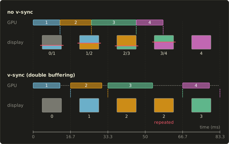
Without v-sync, the buffers are swapped as soon as a frame is done: at 12, 26, 46 and 58 ms.
At 12 ms the display is of the way through its first refresh, so the top 72 % of the screen shows frame 0 and the rest frame 1; on a 1080-line screen the tear is near line .
The other swaps land at , and of their refreshes.
Every refresh has a seam, each time in a different place: that's tearing.
The reward is the lowest latency, because a new frame appears as soon as it exists.
With v-sync and two buffers, a finished frame waits for the next refresh boundary, and the GPU can't start the next frame until the swap frees a buffer.
Frame 1 is shown at 16.7 ms; frame 2 renders from 16.7 to 30.7 ms and is shown at 33.3 ms; frame 3 needs 20 ms (33.3 to 53.3 ms), misses the refresh at 50 ms and appears only at 66.7 ms.
The refresh at 50 ms shows frame 2 a second time.
No tearing, but an uneven rhythm (stutter) and more latency: frame 3 waits 13.3 ms after it was finished.
The usual remedies:
- Triple buffering (トリプルバッファ): a second back buffer lets the GPU start the next frame while a finished one waits for the refresh; the display still shows only whole frames.
- Variable refresh rate (VRR, 可変リフレッシュレート): the display waits for the GPU instead, starting a refresh when a frame is ready (within its supported range). No tearing and no fixed 16.7 ms grid.
Latency
For interaction what matters is latency (遅延, レイテンシ): the time from an input (a mouse move, a button, a head turn) to the changed picture reaching the eye, "input to photon".
Worked example. At 60 Hz, a typical pipelined engine reads the input at the start of a frame, the CPU spends that frame (16.7 ms) on simulation and recording commands, the GPU renders it during the next one (16.7 ms), and the swap happens at the refresh boundary; the display then needs half a refresh (8.3 ms) to scan down to the middle of the screen.
Total: ms, plus the display's own processing; at 120 Hz the same chain takes about 20.8 ms.
Engines shorten it by sampling input as late as possible and limiting how far the CPU may run ahead of the GPU.
Doing less work
The fastest triangle is the one you don't draw:
- view-frustum culling and back-face culling (chapter 6, section 6.4);
- occlusion culling (オクルージョンカリング): skip objects hidden behind others, for example by testing their bounding boxes against a coarse depth buffer, the z-buffer idea of chapter 10 applied to whole objects;
- level of detail (chapter 9, section 9.1) and instancing (many copies of one mesh in a single draw command).
Forward and deferred rendering
- Forward rendering (フォワードレンダリング) shades each fragment completely while drawing its object, looping over the lights that affect it. Simple, and fine with transparency and MSAA, but with many lights and much overdraw the same pixel is lit several times for nothing.
- Deferred rendering (ディファードレンダリング) first draws all opaque geometry into a G-buffer (Gバッファ): per pixel the depth, normal, base color, roughness and so on, without lighting. A second pass lights each visible pixel once, so the cost depends on pixels times lights, not on overdraw.
Worked example. A G-buffer of four 32-bit render targets plus 32-bit depth stores 20 bytes per pixel: at 1920 × 1080 that's bytes, about 41.5 MB.
Written and read once per frame at 60 fps, it costs GB/s.
A G-buffer pixel holds only one surface, so transparent objects are drawn forward afterwards, and MSAA becomes expensive.
Many engines use tiled or clustered shading: lights are sorted into screen tiles or 3D clusters, and each pixel only loops over the lights of its cluster.
Hardware ray tracing
Since 2018, GPUs have units for ray traversal and ray–triangle intersection, used through the ray tracing extensions of Vulkan and Direct3D 12 (chapter 12, section 12.9).
Most games use them in a hybrid way: the primary image is still rasterized, and rays add reflections, shadows or global illumination with a few samples per pixel, cleaned by a denoiser.
Updating the acceleration structures for moving objects must also fit in the frame budget.
Consoles and mobile GPUs
A game console (ゲーム機) is a fixed real-time system: every unit has the same CPU, GPU and unified memory, so a game can be tuned for exactly that hardware.
Mobile GPUs are limited by power and heat, and moving data to external memory costs a lot of energy.
Most therefore use tile-based rendering (タイルベースレンダリング): the screen is divided into small tiles (for example 32 × 32 pixels), the GPU first sorts the frame's triangles into the tiles they touch, then renders one tile at a time in a small on-chip memory, and writes only the finished colors out.
The depth buffer often never leaves the chip.
A 1920 × 1080 screen in 32 × 32 tiles has tiles, and the G-buffer of the previous example can stay on-chip too if the lighting pass reads the same tile.
VR and AR systems
A head-mounted display (HMD, ヘッドマウントディスプレイ) puts displays and lenses in front of the eyes and updates the picture as the head moves.
Its system requirements are tough:
- head tracking (ヘッドトラッキング) with 6 degrees of freedom (6DoF: three rotations, three translations), today mostly inside-out (cameras and inertial sensors on the headset watch the room) rather than outside-in (external sensors watch the headset);
- stereo rendering, two views per frame (section 17.6), which GPUs and APIs can draw in one pass (multi-view);
- high refresh rates: commonly 90 Hz, leaving ms per frame for both eyes;
- low motion-to-photon latency (モーション・トゥ・フォトン遅延), with a target often quoted of about 20 ms or less.
Worked example. Turning your head at 100° per second with 20 ms of lag puts the virtual world away from where it should be; on a display with 20 pixels per degree that's 40 pixels.
The world seems to swim with the head, a classic trigger of VR sickness (section 18.2).
Headsets fight it with prediction (render for where the head will be) and reprojection (re-warp the finished image with the newest head pose just before scan-out).
The lenses add pincushion distortion, so the renderer pre-distorts the image with the opposite barrel distortion; with eye tracking, foveated rendering (フォービエイテッドレンダリング, section 18.5) spends full detail only where the eye is looking.
AR (augmented reality, 拡張現実) overlays CG on the real world, through a transparent display (optical see-through) or on camera video (video see-through); its extra problem is registration (位置合わせ), keeping virtual objects glued to real ones.
Exam points
- Unified shaders: one kind of lane for all shader stages; fixed units for rasterization, texture filtering, ROP, ray tracing.
- fps and ms are reciprocals; budgets add in ms.
- No v-sync: tearing, lowest latency. Double-buffered v-sync: no tearing, but a late frame waits for the next refresh (stutter; 60 fps drops to 30). Triple buffering and VRR soften this.
- Forward: shade while drawing. Deferred: G-buffer first, then light each pixel once (good for many lights, bad for transparency and MSAA).
- Tile-based rendering keeps tiles on-chip to save bandwidth and power.
- VR: 6DoF tracking, stereo rendering, high refresh rate, low motion-to-photon latency.
17.5 3D data input devices
Pointing, drawing and feeling
The everyday input devices of CG are 2D: the mouse (マウス), and the pen tablet (ペンタブレット), which adds absolute position, tilt and pen pressure (筆圧).
Pressure is quantized like any measurement (chapter 2, section 2.5): many tablets report 8,192 levels, , a 13-bit value that drives brush size or opacity.
A 3D mouse (3Dマウス) is a puck that can be pushed, pulled, tilted and twisted, six degrees of freedom for flying the camera with one hand.
A haptic device (力覚提示装置) is a small robot arm with a pen that pushes back when the virtual tool touches a surface; force feedback needs a fast loop (around 1,000 updates per second is a commonly used rate), or hard surfaces feel soft.
Motion capture is covered in chapter 13.
To bring the shape of a real object into the computer we need a 3D scanner (3Dスキャナー, 3次元形状計測装置).
Kinds of 3D scanner
| Active (能動型) | Passive (受動型) | |
|---|---|---|
| Idea | projects its own light (laser, pattern, pulse) | uses only the existing light, like a camera |
| Methods | laser triangulation, structured light, time of flight, LiDAR | stereo, photogrammetry |
| Strengths | works on plain, untextured surfaces; dense and precise | cheap (just cameras), any distance, captures color |
| Weaknesses | sunlight can drown the signal | needs surface texture to find matches |
The other division is contact (接触式) versus non-contact (非接触式).
A coordinate measuring machine (CMM, 三次元測定機) touches the object with a probe on a precise arm: accurate to micrometers, but slow, point by point, and only for objects that may be touched.
All the optical methods below are non-contact, and all struggle with shiny, transparent or very dark surfaces, which don't send the light back to the sensor in a predictable way.
Laser triangulation
A laser projects a dot or a line onto the object, and a camera at a known distance from the laser sees where it lands.
Laser, camera and lit point form a triangle with one known side and two known angles, hence triangulation (三角測量); laser-line scanners are also called 光切断法 (light-section method), because the line "cuts" the object and its bent image shows the profile.
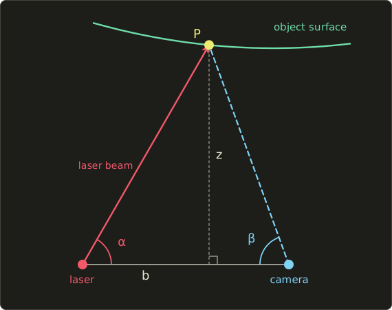
Put the laser at the origin and the camera at distance (the baseline, 基線長) along the x axis.
The beam leaves at the known angle ; the camera measures the angle from the dot's pixel position (the pinhole model of chapter 2, section 2.2).
If the point is at , the two right triangles under it give and , so
(multiply top and bottom by and use ).
Worked example. mm, , .
- , , sum .
- mm, and mm.
- Check: mm.
A longer baseline makes the depth more precise, but the camera then sees the object from a more different direction, and more points are hidden from either the laser or the camera (occlusion: holes in the scan).
Triangulation is very precise at short range and is used for small objects, inspection and dental scanning.
Structured light
A structured-light scanner (パターン投影法) replaces the laser with a projector and lights the whole object with a series of patterns, photographed by a camera.
Each projector column gets a unique code, so each camera pixel can find out which column lit it, and triangulation does the rest.
With black-and-white stripe patterns, each column receives an -bit code and columns can be told apart: 10 patterns identify 1,024 stripes.
The codes are usually Gray codes (グレイコード), in which neighboring stripes differ in exactly one bit, so a misread pixel on a stripe boundary is off by at most one stripe:
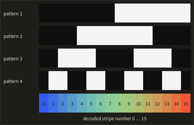
Read the four patterns from top to bottom at one column (black = 0, white = 1) and you get its code; stripe 5, for example, reads 0, 1, 1, 1.
This is called space coding (空間コード化法); finer precision comes from phase shifting (位相シフト法), a few shifted sinusoidal patterns that give each pixel a continuous position within its stripe.
Time of flight and LiDAR
A time-of-flight (ToF) sensor measures how long light takes to reach the object and come back.
Light travels m/s, about 30 cm per nanosecond, and it covers the distance twice:
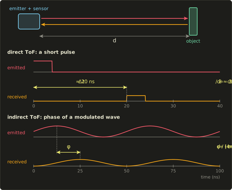
Direct ToF times the echo of a short pulse:
Worked example. ns: m.
To resolve 1 mm, the clock would need picoseconds, which is why direct ToF suits longer ranges, where centimeters are good enough.
Indirect ToF modulates the light's brightness at a frequency (tens of MHz) and measures the phase shift between the emitted and the received wave.
One full period corresponds to a round trip of , so
Worked example. MHz (period 50 ns), (a quarter period, 12.5 ns): m.
The phase repeats every , so the distance is unambiguous only up to m; an object at m gives the same phase, and sensors combine several frequencies to extend the range.
LiDAR (ライダー) is ToF with a scanning laser that measures millions of points per second over long distances: surveying from aircraft and drones, self-driving cars, building scans, and small solid-state versions in some phones and tablets.
Stereo and depth from disparity
Stereo (ステレオ法) is passive triangulation: two cameras replace the laser and the camera.
A point appears at slightly different positions in the two images, and that difference, the disparity (視差), tells its depth, as binocular disparity does for our eyes (chapter 3, section 3.9).
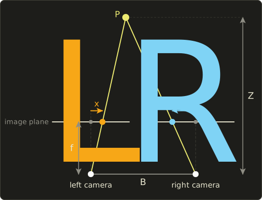
Take two identical pinhole cameras with parallel axes, a baseline apart, focal length .
A point at horizontal position (from the left camera) and depth projects to in the left image and in the right one, each measured from that camera's image center.
Subtract:
Depth is inversely proportional to disparity: near points have large disparities, a point at infinity has .
In the figure, , , : , , , and indeed .
Worked example in pixels. A 4 mm lens with 4 µm pixels gives pixels; the baseline is m.
A disparity of 40 pixels means m; 39 pixels would mean m.
Differentiating gives the depth error for a disparity error :
At 3 m that's m per pixel; at 6 m (disparity 20) it's m, four times worse at twice the distance.
Stereo precision falls with the square of the distance; a wider baseline or longer focal length helps.
The hard part is the correspondence problem (対応点探索): which pixel in the right image shows the same point as a given pixel in the left one?
Calibrated images are first rectified (平行化) so that matching points lie on the same row, then a matcher compares small windows along that row.
Matching fails on textureless surfaces (a white wall looks the same everywhere), repeating patterns and shiny materials; active stereo projects a random dot pattern to give every surface texture.
Photogrammetry and depth cameras
Photogrammetry (フォトグラメトリ) extends stereo to many photos from unknown positions (chapter 9, section 9.5): structure from motion (SfM) matches features across the photos and solves for the camera positions and a sparse point cloud together, then multi-view stereo (MVS) builds a dense point cloud and a textured mesh.
Only a camera is needed and the color comes for free (chapter 12, section 12.13, calls this image-based modeling).
One trap: photos alone can't tell the scale (a toy house up close looks like a real house farther away), so a known length must be added, such as a scale bar.
Depth cameras (深度カメラ) deliver a whole depth image at video rate with one of the active principles: structured light, indirect ToF or active stereo (a depth sensor sold for a game console in 2010 used structured light, its successor ToF).
They are cheap and fast but noisier than dedicated scanners: gesture input, robotics, AR room mapping, quick scans.
From point cloud to mesh
A scanner delivers a point cloud (点群) or depth images, not yet a usable model:
- Registration (位置合わせ): scans from different viewpoints are aligned roughly (by hand or with markers), then precisely with ICP (iterative closest point), which repeatedly pairs each point with its nearest neighbor in the other scan and solves for the rigid transform that brings the pairs closest.
- Merging and cleaning: overlaps are combined, outliers and noise removed.
- Surface reconstruction: for example Poisson reconstruction, or the zero isosurface of a signed-distance volume extracted with marching cubes (section 9.3).
- Repair: holes are filled, and the mesh is made watertight for printing (section 17.7).
- Simplification and texturing: the mesh is reduced or rebuilt, detail is baked into normal maps (chapter 11), and the photos become the color texture.
Exam points
- Active methods project light (laser triangulation, structured light, ToF, LiDAR); passive ones only use cameras (stereo, photogrammetry). Contact (CMM) vs non-contact.
- Triangulation: ; a longer baseline means more precision but more occlusion.
- Structured light: Gray-code patterns identify stripes; neighbors differ in one bit.
- ToF: (pulse) or (phase, ambiguous beyond ).
- Stereo: ; the error grows with ; needs texture for correspondences. Photogrammetry: SfM then MVS; scale needs a known length.
17.6 Output devices: displays and stereoscopic display
Display technologies
- An LCD (液晶ディスプレイ) is a grid of light valves in front of a backlight: the liquid crystal turns the light's polarization so that more or less of it passes a second polarizer, and color filters make the subpixels. The backlight is always on, so black is never fully black; local dimming (separately dimmed LED zones) improves contrast.
- An OLED display (有機EL) is self-emissive: each subpixel is a tiny organic LED, and black pixels are simply off. Very high contrast and fast response; the materials age, so static images can burn in.
- Micro-LED (マイクロLED) is also self-emissive, with tiny inorganic LEDs: bright and long-lived, but at the time of writing hard to manufacture except for large modular video walls.
The main numbers:
- Resolution (解像度): 1920 × 1080 (Full HD), 3840 × 2160 (4K UHD), 7680 × 4320 (8K). The eye sees pixel density: a 27-inch 4K monitor has pixels per inch.
- Refresh rate (リフレッシュレート): 60 Hz for most TVs and office monitors, 120 to 240 Hz and more for gaming, 90 Hz and up in VR.
- Response time (応答速度): how fast a pixel changes. Slow pixels smear motion, and even instant pixels that hold their value for the whole refresh look blurred to an eye following a moving object (section 18.3).
- Gamut and HDR: wide-gamut displays cover DCI-P3 or part of BT.2020 (chapter 3, section 3.4). An HDR display (HDRディスプレイ) has a much higher peak luminance (hundreds to thousands of cd/m², "nits") and deeper blacks, and takes 10-bit signals with a perceptual transfer curve such as PQ (defined up to 10,000 cd/m²) or HLG instead of the sRGB curve of section 3.7.
Projectors (プロジェクタ) form the image on a small LCD, LCoS or DLP chip; a DLP chip (DMD, digital micromirror device) has millions of tiny mirrors that flip on and off thousands of times per second, the fraction of time "on" giving the brightness.
Projecting onto buildings or objects with the image pre-warped to their shape is projection mapping (プロジェクションマッピング).
The cable to the display limits resolution × refresh rate × bit depth: at the time of writing HDMI 2.1 carries up to 48 Gbit/s, HDMI 2.2 (2025) up to 96 Gbit/s and DisplayPort 2.1 up to 80 Gbit/s, part of which goes to line coding and blanking.
Worked example. 4K at 120 Hz with 10 bits per channel needs Gbit/s of raw pixel data and fits a 48 Gbit/s link; 4K at 240 Hz needs Gbit/s and doesn't, so it needs Display Stream Compression (DSC) or a faster link.
Stereoscopic display
To show depth through binocular disparity, each eye must get its own image: a stereoscopic display (立体ディスプレイ).
The two images come from two virtual cameras one interpupillary distance (IPD, 瞳孔間距離) apart, about 63 mm on average for adults.
They should look in parallel directions, each with an asymmetric (off-axis) frustum framing the same screen rectangle (the general perspective matrix of Linear Algebra chapter 12 with unequal left and right planes), not "toe-in" (cameras rotated towards one point), which causes unwanted vertical disparities in the corners.
On the screen a point appears twice; the horizontal distance between the two is the screen parallax (スクリーン視差) .
For eyes apart at distance from the screen, a point at distance from the viewer has, by similar triangles,
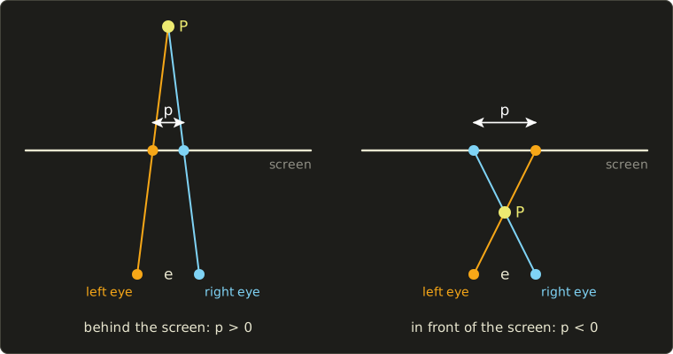
Worked example. mm, m.
- m (behind the screen): mm, positive or uncrossed parallax (非交差視差).
- m: , the point appears on the screen.
- m (in front): mm, negative or crossed parallax (交差視差).
- : . Parallax above would force the eyes to diverge, so stereo content keeps it within limits.
(The figure shows the same two cases, and , with the eye separation exaggerated.)
How the two images are separated defines the type of display:
- Anaglyph (アナグリフ): one image in red, the other in cyan, viewed through red/cyan glasses. Works on any screen or paper, but colors suffer. As a shader it's one line:
// Red-cyan anaglyph: red from the left eye's image, green and blue from the right eye's.
float3 anaglyph(float3 left, float3 right) {
  return float3(left.r, right.g, right.b);
}
// Red-cyan anaglyph: red from the left eye's image, green and blue from the right eye's.
vec3 anaglyph(vec3 left, vec3 right) {
return vec3(left.r, right.g, right.b);
}// Red-cyan anaglyph: red from the left eye's image, green and blue from the right eye's.
float3 anaglyph(float3 left, float3 right) {
return float3(left.r, right.g, right.b);
}
- Polarized glasses (偏光方式, passive): the two images leave with different polarizations (two filtered projectors, or alternate display rows behind a patterned filter), and each lens of the glasses passes only one. Common in cinemas; with alternate rows each eye gets half the vertical resolution.
- Active shutter glasses (液晶シャッター方式, time division): the display alternates left and right images, and liquid-crystal shutters in the glasses, synchronized with it, block the other eye. Full resolution, but half the frames per eye: 120 Hz becomes 60 Hz per eye.
- Autostereoscopic displays (裸眼立体視) need no glasses. A parallax barrier (視差バリア) is a layer of thin slits a small distance in front of the pixels, so that from the left eye only the "L" columns are visible and from the right eye only the "R" columns; a lenticular sheet (レンチキュラーレンズ) uses tiny cylindrical lenses instead, which waste less light.
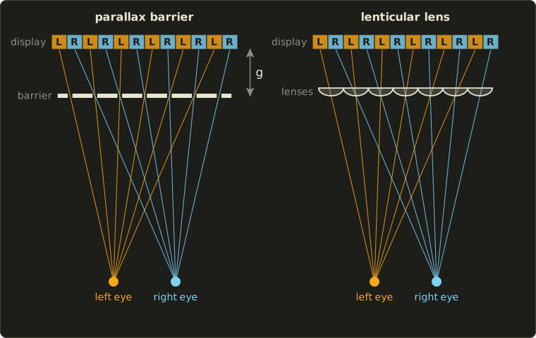
Through one slit, the two eyes must see two neighboring columns, a column pitch apart.
By similar triangles , so the gap is ; in the figure , , give and a slit pitch of , slightly less than two columns.
For a real panel with 0.1 mm columns, mm and mm: mm.
The price: it works only from certain viewing positions, and each eye gets a fraction of the columns; multi-view displays use more than two views so the image changes as the viewer moves.
- Head-mounted displays (section 17.4) give each eye its own image, and head tracking adds motion parallax. Like every stereo screen they cause the vergence–accommodation conflict (the eyes converge on the virtual distance but focus at the fixed optical distance), explained in section 18.2.
- Holography (ホログラフィ) records and reproduces the light's wavefront through interference patterns, so it provides all depth cues, including focus. Computer-generated holograms need pixels near the wavelength of light and enormous pixel counts, so at the time of writing they're mostly research; light-field displays, which send different images in many directions, sit between multi-view displays and holograms.
Exam points
- LCD: backlight plus light valves; OLED and micro-LED: self-emissive.
- Refresh rate, response time, resolution, pixel density, gamut, HDR (peak luminance, 10 bits, PQ/HLG).
- Stereo pairs: two cameras one IPD apart, parallel axes, off-axis frusta; : positive behind the screen, zero on it, negative in front.
- Glasses: anaglyph (color), polarized (passive), shutter (time division). No glasses: parallax barrier, lenticular. HMD: vergence–accommodation conflict. Holography reproduces the wavefront.
17.7 Printers and 3D printers
2D printers and halftoning
Inkjet printers (インクジェットプリンタ) shoot tiny droplets of the subtractive CMYK inks of chapter 3 (section 3.3), pushed out by heat or by a piezoelectric element.
Laser printers (レーザープリンタ) draw the page as electric charge on a drum with a laser; the charged areas pick up toner, which is fused onto the paper.
Dye-sublimation printers (昇華型プリンタ) heat dye from a ribbon into the paper in continuously varying amounts: true continuous tone, for photo prints.
Inkjet and laser printers can only put a dot or leave the paper white.
Gray levels and mixed colors come from halftoning (ハーフトーン, 網点): small dots whose average covers the right fraction of the paper, the idea behind the dithering of chapter 2 (section 2.8).
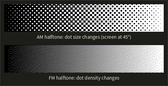
- AM screening (AMスクリーニング): dots on a regular grid (the screen) grow and shrink. The grid spacing is the screen ruling in lines per inch (lpi).
- FM screening (FMスクリーニング): all dots have the same small size and their density changes; error diffusion is one way to place them.
Worked example. A 600 dpi printer builds each halftone cell from 8 × 8 printer dots.
The screen ruling is lpi, and a cell can have 0 to 64 dots set: gray levels.
Smaller cells show more detail but fewer levels; that trade-off is the core of AM halftoning.
In color printing the four screens are rotated to different angles (traditionally about 15°, 75°, 0° and 45° for C, M, Y and K), because screens at similar angles would interfere into visible moiré.
3D printers: additive manufacturing
A 3D printer (3Dプリンタ) builds a solid object layer by layer from a digital model: additive manufacturing (付加製造), in Japanese usually 積層造形.
The standard terminology (ISO/ASTM 52900) sorts the processes into seven categories; these four are the ones you meet most in CG work:
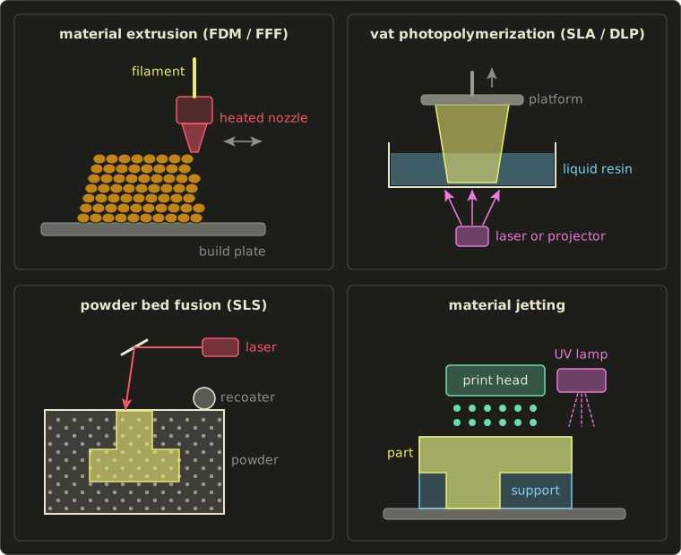
| Category | Typical names | How it works | Notes |
|---|---|---|---|
| Material extrusion (材料押出) | FDM, FFF (熱溶解積層法) | a heated nozzle melts plastic filament and lays it down in beads | cheap and common; visible layer lines; overhangs need supports |
| Vat photopolymerization (液槽光重合) | SLA (光造形法), DLP, LCD | light cures liquid resin one layer at a time: a laser traces each layer (SLA), or a projector or LCD exposes the whole layer at once | smooth, fine detail; supports, washing and post-curing |
| Powder bed fusion (粉末床溶融結合) | SLS (粉末焼結法); SLM, DMLS for metal | a recoater spreads powder, a laser fuses the cross-section, repeat | loose powder supports overhangs, so polymer parts need no supports; metal parts |
| Material jetting (材料噴射) | inkjet 3D printing | print heads jet droplets of photopolymer, cured at once by UV light | several materials and full color in one part; dissolvable supports |
The other three categories are binder jetting (a liquid binder glues powder), directed energy deposition (material melted as it's fed, for metal) and sheet lamination.
From mesh to layers
A printer can only build a real solid, so the model must be the closed, consistently oriented, manifold mesh of chapter 7 (section 7.4); a hole or self-intersecting parts leave "inside" undefined.
It's exported as STL (triangles only, no units, chapter 9, section 9.1) or, better, 3MF, a zipped XML format that also stores units, colors, materials and several objects.
A slicer (スライサー) cuts the mesh with horizontal planes, one per layer, and turns each cross-section into machine instructions (G-code toolpaths for FDM): outer walls, an inner infill (インフィル) pattern that saves material, and supports (サポート) under overhangs.
An edge from to with crosses the plane at
Worked example. The edge from to mm at mm: , .
Each triangle straddling the plane yields one segment, and in a watertight mesh the segments join into closed loops, the outlines of the layer; with a hole, a loop stays open and the slicer can't tell inside from outside.
Layer thickness sets vertical resolution and time.
A 60 mm tall part at 0.2 mm per layer needs layers; a DLP printer exposing each layer in 7.5 s (including the peel movement) needs s = 37.5 minutes, whether one part or twenty are on the platform, while FDM and laser SLA must trace every outline, so their time grows with the amount of material.
Sloped surfaces show a staircase effect with steps one layer high.
The opposite, subtractive manufacturing, removes material from a block: CNC milling (切削加工) moves a rotating cutter along toolpaths computed from the model, on 3 axes or 5 (the cutter also tilts).
It gives precise, strong parts, but a 3-axis mill can't cut undercuts or closed internal cavities, which additive methods build easily.
Exam points
- Halftoning: AM (dot size on a fixed screen, lpi), FM (dot density); an cell gives levels at dpi / lpi.
- FDM/FFF: melted filament from a nozzle. SLA: laser cures resin; DLP: projector cures a whole layer. SLS: laser fuses powder, the powder supports overhangs. Material jetting: inkjet droplets, UV cured, multi-material.
- Printable meshes are watertight and manifold; STL has no units, 3MF has units and materials; slicers add supports and infill.
- Additive (layers) vs subtractive (CNC milling).
17.8 Recording media
The kinds of media
Recording media (記録メディア) differ in how they store bits, and so in capacity, speed, cost and lifetime:
| Medium | How bits are stored | Capacity (at the time of writing) | Speed and access | Typical use |
|---|---|---|---|---|
| HDD | magnetic regions on spinning platters | up to a few tens of TB per drive | a few hundred MB/s sequential at best; milliseconds to seek | bulk storage, servers |
| SSD | charge in NAND flash cells, no moving parts | several TB in PCs | SATA about 0.5 GB/s, NVMe several GB/s; fast random access | system and project drives |
| Memory cards | NAND flash (SD family, CFexpress) | by specification SDHC up to 32 GB, SDXC up to 2 TB, SDUC up to 128 TB | depends on the card class | cameras, phones |
| Optical discs | pits or marks read by a laser | CD 700 MB; DVD 4.7 GB (8.5 GB dual layer); Blu-ray 25 GB (50 GB dual layer), BDXL 100 or 128 GB | slow; removable; write-once versions | distribution, small archives |
| Magnetic tape (LTO) | magnetic tape in a cartridge | LTO-9 18 TB; LTO-10 30 or 40 TB (native) | fast streaming, but sequential access only | backup, long-term archives |
| Cloud storage | data centers over the network | practically unlimited, paid per GB | limited by the network | sharing, off-site backup |
Optical discs became denser mainly through shorter laser wavelengths, which focus to smaller spots: about 780 nm for CD, 650 nm for DVD and 405 nm (blue-violet) for Blu-ray, hence its name.
Tape is the cheapest medium per terabyte, lasts for decades on a shelf, uses no power there and is out of reach of network attacks.
Tape capacities are also printed for 2.5:1 compression (LTO-10: 75 or 100 TB); for already compressed images and video the native number is the honest one.
Capacity and bandwidth arithmetic
Worked example: uncompressed 4K video. 3840 × 2160 pixels, 8-bit RGB, 24 frames per second:
- one frame: bytes, about 24.9 MB;
- one second: bytes, about 597 MB/s;
- one minute: GB.
So a 25 GB Blu-ray holds seconds of it, and an 18 TB LTO-9 tape minutes.
597 MB/s is more than one hard disk or one LTO-10 drive (400 MB/s native) can write, so real-time playback needs fast SSDs or several disks in parallel (RAID).
Compressed at 50 Mbit/s, a minute is MB: a ratio of about .
Codecs and containers
A codec (コーデック) is a compression method for video or audio.
Video codecs use the JPEG ideas of chapter 2 (section 2.10) inside each frame (intra-frame coding: YCbCr, chroma subsampling, transform, quantization) and add inter-frame coding: most of a frame is predicted from neighboring frames by motion compensation (動き補償), and only the difference is stored.
Self-contained frames are I-frames; predicted ones are P-frames (from earlier frames) and B-frames (from earlier and later ones).
The well-known generations are H.264/AVC (2003, the most compatible), H.265/HEVC (2013, similar quality at roughly half the bit rate, used for 4K and HDR) and AV1 (2018, Alliance for Open Media, royalty-free, widely used for streaming).
A container (コンテナ) is the file format that holds compressed video, audio and subtitles together: MP4, MOV, MKV.
Container and codec are independent: an .mp4 file can hold H.264, HEVC or AV1.
Production keeps working files as image sequences (one OpenEXR or DPX file per frame) or in intra-only codecs, so that every frame stays editable at full quality; strongly compressed inter-frame codecs are for delivery.
Long-term archiving
Keeping data readable for decades is hard: media decay (bits silently flip), drives disappear (think of floppy disks), and formats become unreadable when their software is gone, so open, documented formats (OpenEXR, PNG, glTF, USD) age better than proprietary ones.
Long-term archiving (長期保存) therefore stores checksums to detect damage, migrates data to new media and formats regularly, and keeps several copies, often by the 3-2-1 rule: three copies, on two kinds of media, one off-site.
Exam points
- Magnetic (HDD, tape), optical (CD, DVD, Blu-ray), semiconductor (SSD, memory cards), network (cloud); shorter wavelength → denser optical disc.
- Tape: sequential, cheap per TB, for backup and archives; SSD: fast random access.
- Uncompressed video size = width × height × bytes per pixel × fps × seconds.
- Codec (compression) vs container (file format); intra-frame vs inter-frame coding (motion compensation).
17.9 Summary
- A CG system has input, processing, output and storage. CPUs are latency-oriented, GPUs throughput-oriented SIMT machines limited by memory bandwidth; render farms parallelize by frame.
- Software: DCC tools, sculpting, CAD, renderers, compositing, image editing and game engines, connected by OBJ, FBX, glTF, USD, Alembic and STL/3MF; graphics APIs differ from shading languages.
- Real-time systems count milliseconds: no v-sync tears, double-buffered v-sync stutters, triple buffering and VRR help; culling, LOD, deferred and tile-based rendering save work and bandwidth; VR adds 6DoF tracking, stereo, high refresh rates and low latency.
- 3D input: contact or non-contact, active (triangulation, structured light, ToF , LiDAR) or passive (stereo , photogrammetry) scanners; point clouds become meshes by registration, reconstruction and repair.
- Output: LCD, OLED and micro-LED displays, projectors, stereo displays with screen parallax (glasses, autostereoscopic, HMDs), halftoning printers, 3D printers building watertight sliced meshes layer by layer, and CNC milling.
- Media: HDD, SSD, memory cards, optical discs, LTO tape and cloud; video codecs inside containers; archives need checksums, migration and several copies.
17.10 Key terms
| English | 日本語 |
|---|---|
| CG system | CGシステム |
| CG software | CG用ソフトウェア |
| real-time 3D CG system | リアルタイム3次元CGシステム |
| 3D data input device | 3次元データ入力装置 |
| 3D data output device | 3次元データ出力装置 |
| recording media | 記録メディア |
| latency, throughput | レイテンシ(遅延)、スループット |
| SIMT, warp | SIMT、ワープ |
| branch divergence | 分岐ダイバージェンス |
| VRAM, memory bandwidth | VRAM(ビデオメモリ)、メモリ帯域幅 |
| render farm, cloud rendering | レンダーファーム、クラウドレンダリング |
| asset management, version control | アセット管理、バージョン管理 |
| DCC tool, game engine | DCCツール、ゲームエンジン |
| plug-in, scripting | プラグイン、スクリプト |
| graphics API, shading language | グラフィックスAPI、シェーディング言語 |
| middleware | ミドルウェア |
| unified shader architecture | ユニファイドシェーダーアーキテクチャ |
| frame rate, frame time | フレームレート、フレームタイム |
| tearing, v-sync | テアリング、垂直同期 |
| double buffering, triple buffering | ダブルバッファ、トリプルバッファ |
| variable refresh rate (VRR) | 可変リフレッシュレート(VRR) |
| occlusion culling | オクルージョンカリング |
| forward rendering, deferred rendering | フォワードレンダリング、ディファードレンダリング |
| G-buffer | Gバッファ |
| tile-based rendering | タイルベースレンダリング |
| head-mounted display (HMD) | ヘッドマウントディスプレイ(HMD) |
| head tracking, 6DoF | ヘッドトラッキング、6自由度(6DoF) |
| motion-to-photon latency | モーション・トゥ・フォトン遅延 |
| foveated rendering | フォービエイテッドレンダリング |
| augmented reality (AR) | 拡張現実(AR) |
| pen tablet, pen pressure | ペンタブレット、筆圧 |
| haptic device | 力覚提示装置(ハプティックデバイス) |
| 3D scanner | 3Dスキャナー(3次元形状計測装置) |
| contact, non-contact | 接触式、非接触式 |
| coordinate measuring machine (CMM) | 三次元測定機 |
| active, passive | 能動型(アクティブ)、受動型(パッシブ) |
| triangulation, baseline | 三角測量、基線長 |
| light-section method | 光切断法 |
| structured light | パターン投影法 |
| Gray code, space coding | グレイコード、空間コード化法 |
| phase shifting | 位相シフト法 |
| time of flight (ToF) | TOF(Time of Flight)方式 |
| LiDAR | ライダー(LiDAR) |
| stereo, disparity | ステレオ法、視差 |
| correspondence problem, rectification | 対応点探索、平行化 |
| structure from motion (SfM), multi-view stereo (MVS) | SfM、多視点ステレオ(MVS) |
| depth camera | 深度カメラ(デプスカメラ) |
| registration (of scans) | 位置合わせ |
| liquid crystal display (LCD), OLED | 液晶ディスプレイ、有機EL |
| refresh rate, response time | リフレッシュレート、応答速度 |
| HDR display | HDRディスプレイ |
| projector, projection mapping | プロジェクタ、プロジェクションマッピング |
| stereoscopic display | 立体ディスプレイ(立体視) |
| interpupillary distance (IPD) | 瞳孔間距離 |
| screen parallax (crossed, uncrossed) | スクリーン視差(交差視差、非交差視差) |
| anaglyph | アナグリフ |
| polarized glasses, active shutter glasses | 偏光方式、液晶シャッター方式 |
| autostereoscopic display | 裸眼立体視ディスプレイ |
| parallax barrier, lenticular lens | 視差バリア(パララックスバリア)、レンチキュラーレンズ |
| holography | ホログラフィ |
| halftoning, AM / FM screening | ハーフトーン(網点)、AM/FMスクリーニング |
| 3D printer, additive manufacturing | 3Dプリンタ、積層造形(付加製造) |
| material extrusion (FDM/FFF) | 材料押出(熱溶解積層法) |
| vat photopolymerization (SLA/DLP) | 液槽光重合(光造形法) |
| powder bed fusion (SLS) | 粉末床溶融結合(粉末焼結法) |
| material jetting | 材料噴射(マテリアルジェッティング) |
| slicer, support, infill | スライサー、サポート、インフィル |
| CNC milling | 切削加工(CNC) |
| HDD, SSD, memory card | ハードディスク(HDD)、SSD、メモリカード |
| optical disc (CD, DVD, Blu-ray) | 光ディスク(CD、DVD、ブルーレイ) |
| magnetic tape (LTO) | 磁気テープ(LTO) |
| cloud storage | クラウドストレージ |
| codec, container | コーデック、コンテナ |
| intra-frame, inter-frame coding | フレーム内符号化、フレーム間符号化 |
| motion compensation | 動き補償 |
| long-term archiving | 長期保存(アーカイブ) |
17.11 Challenges
- ★ A direct ToF sensor receives an echo after 40 ns. How far is the object, and how much distance does a timing error of 1 ns correspond to? An indirect ToF sensor at MHz measures : compute the distance and the unambiguous range.
- ★ A stereo camera has pixels and m. Compute the depth for disparities of 40, 20 and 10 pixels, and the depth error for a one-pixel disparity error at each. What happens to the error when the distance doubles?
- ★ Ten minutes of uncompressed 1920 × 1080 video, 8-bit RGB, 60 frames per second: how many GB is it, how many 50 GB Blu-ray discs would it fill, and what fraction of an 18 TB LTO-9 tape? How big is it at 20 Mbit/s?
- ★★ A 60 Hz display and a GPU whose frames take 10, 18, 15 and 25 ms, starting at 0 ms. Without v-sync, at what fraction of the screen height does each swap tear? With double-buffered v-sync, when is each frame shown, and which refreshes repeat an old frame?
- ★★★ A deferred renderer at 1920 × 1080 and 60 fps uses a 20-byte-per-pixel G-buffer written once and read once per frame. Compute the bandwidth, explain why a tile-based mobile GPU can avoid most of it, and explain why transparent objects can't simply be put into the G-buffer.
Multiple choice
Q1 ★ Which of the following statements about 3D data input is correct?
| A | A time-of-flight sensor finds the distance from the angle between the laser beam and the camera's line of sight. |
| B | Photogrammetry is an active method: it projects stripe patterns onto the object and photographs them. |
| C | A coordinate measuring machine (CMM) measures objects without touching them, using a laser. |
| D | In stereo, depth is inversely proportional to disparity, so the depth error for a one-pixel disparity error grows roughly with the square of the distance. |
| E | In stereo, the farther away a point is, the larger its disparity between the two images. |
Q2 ★ Which of the following statements about tearing and v-sync is correct?
| A | Tearing is caused by double buffering with v-sync turned on when the GPU renders too slowly. |
| B | V-sync swaps the front and back buffers while the display is scanning the middle of the screen. |
| C | With double-buffered v-sync on a 60 Hz display, a frame that takes 20 ms to render is shown 20 ms after it was started. |
| D | Triple buffering removes the need for a back buffer. |
| E | With a variable refresh rate, the display starts a refresh when the GPU has finished a frame (within the range it supports), which reduces both tearing and stutter. |
Q3 ★★ Which of the following statements about 3D printing is correct?
| A | FDM (fused deposition modeling) builds the object by curing liquid resin with ultraviolet light. |
| B | In powder bed fusion (SLS), a laser fuses layers of powder, and the unfused powder holds up overhangs, so polymer parts usually need no separate supports. |
| C | A DLP printer traces each layer point by point with a laser beam, so its printing time grows with the number of parts on the platform. |
| D | Material jetting pushes molten plastic filament out of a heated nozzle. |
| E | STL files store units, colors and materials, so a mesh with holes can still be printed correctly. |
17.12 Practical assignment
Build three "machines" of this chapter on paper, a laser scanner, a stereo camera and a 3D printer's slicer, and check each against exact answers.
You need graph paper (1 cm squares), a ruler, a protractor, a pencil, two colored pens and a calculator.
Part A: laser triangulation.
- Draw a baseline 10 cm long: the laser at and the camera at , in cm.
- Mark three surface points , , , and draw the laser beam from and the camera ray from to each.
- Measure at and at for each point with the protractor, to the nearest degree.
- Compute and from your measured angles, and compare with the true coordinates.
- Repeat step 4 for with wrong by 1° (once larger, once smaller). How much does change?
Part B: a stereo camera.
- Draw two pinholes at and (baseline cm) and the image line above them (focal length cm, image in front of the pinholes as in the stereo figure). Mark each camera's image center at and on that line.
- Mark three points at with depths , and cm, draw the rays from each to both pinholes, and mark where they cross the image line.
- Measure and with the ruler (from each image center, positive to the right), and compute and .
Part C: slicing a pyramid.
A square pyramid has its base from to cm and its apex at cm.
- Slice it at (the centers of 1 cm layers): intersect the edge from to the apex with the formula of section 17.7, use the symmetry to get each square cross-section, and draw the six squares nested in one picture.
- Volume. Treat each layer as a 1 cm slab with the cross-section at its center height, add up the slab volumes and compare with the exact volume . Repeat with the cross-sections at the bottoms of the layers ().
How to check yourself:
- Part A: the true angles are , for ; , for ; , for . Your computed must land within a few millimeters of 6, 8 and 5 cm, and within a few millimeters of 4, 6 and 5 cm.
- Part B: must equal cm² for every point (up to drawing accuracy); the disparities are 3, 1.5 and 1 cm, so tripling the distance cuts the disparity to a third.
- Part C: the edge point at height is , so the cross-section is a square of side ; the center-height slabs add up to 71.5 cm³, within 1 % of the exact 72 cm³, while the bottom-height slabs give 91 cm³. Thinner layers bring both closer to 72.
コメント(0)
まだコメントはありません。
ログインするとコメント出来ます。