6. The Viewing and Drawing Pipelines
In chapter 5 we built the individual pieces: modeling transforms, the view transform and projection.
In this chapter I'll put them on one conveyor belt and run a vertex all the way from a model file to a pixel, with real numbers at every stop.
Then we'll look at what happens to everything that doesn't fit on the screen (clipping and culling), at the stages a GPU goes through to draw a frame, and finally at the classic algorithms that turn lines, circles and polygons into pixels.
Why does this matter?
Every real-time renderer, from a phone game to a CAD viewer, is built around exactly this pipeline, and when something goes wrong (a triangle vanishes, the picture is upside down, the edges of two triangles flicker) you can only find the bug if you know which stage does what.
For the exam, this chapter covers two syllabus items of area 2, viewing pipeline (ビューイングパイプライン) and drawing pipeline (描画パイプライン), including clipping, culling and rasterization.
6.1 Two pipelines
A pipeline is a chain of stages where the output of one stage is the input of the next, like an assembly line.
CG talks about two of them, and they look at the same process from two angles:
| Pipeline | Question it answers | Main contents |
|---|---|---|
| viewing pipeline (ビューイングパイプライン) | Through which coordinate systems does a point travel to reach the screen? | modeling, view and projection transforms, clipping, perspective division, viewport transform |
| drawing (rendering) pipeline (描画パイプライン) | What work does the hardware do to turn triangles into a finished image? | vertex processing, primitive assembly, clipping, rasterization, fragment processing, tests, frame buffer |
The viewing pipeline is mathematics: a sequence of coordinate transformations.
The drawing pipeline is the machine that carries it out, plus everything that comes after the geometry: deciding which pixels a triangle covers and what color they get.
The geometry half of the drawing pipeline is the viewing pipeline, so we'll start there.
6.2 The viewing pipeline, one vertex at a time
Here is the whole chain.
Each box is a coordinate system, each arrow an operation, and the numbers on the right belong to the one vertex we're about to follow.
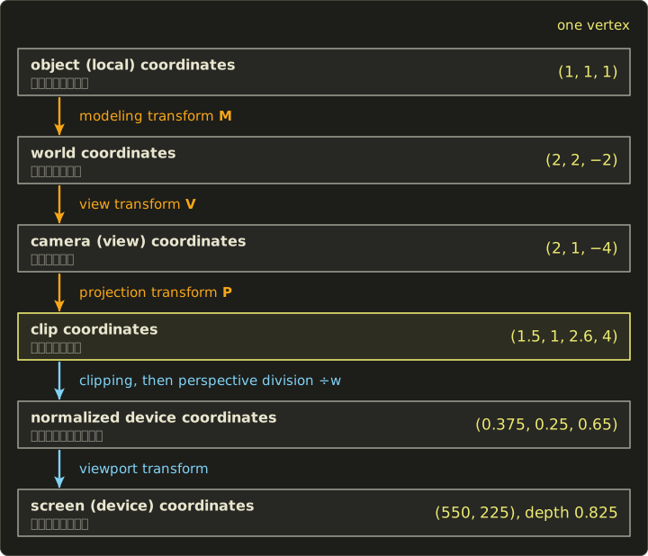
You met most of these spaces in Linear Algebra chapter 11, and the projection matrices are derived in Linear Algebra chapter 12.
I won't derive them again here; this section is about the order and the meaning of each stop:
- Object (local), world and camera (view) coordinates (モデリング座標系 or ローカル座標系, ワールド座標系, カメラ座標系 or 視点座標系): as in chapter 5, the model's own space, the shared scene, and the eye at the origin looking down −Z.
- Clip coordinates (クリップ座標系): 4D homogeneous coordinates right after projection, before any division.
- Normalized device coordinates, NDC (正規化デバイス座標系): after dividing by w, everything visible lies in a fixed cube.
- Screen (device) coordinates (スクリーン座標系, デバイス座標系): pixels of the actual window.
The operations between them are the modeling transform (モデリング変換), the view transform (ビュー変換, also 視野変換), the projection transform (投影変換), clipping (クリッピング), perspective division (透視除算) and the viewport transform (ビューポート変換).
The setup
Our model is a cube with corners at ±1, and we'll follow its corner .
The scene is set up like this:
- Modeling transform: turn the cube 90° around Y, then move it to : .
- Camera: eye , looking at the target , up .
- Projection: perspective (OpenGL convention), vertical field of view 90°, aspect ratio 4/3, near plane , far plane .
- Window: 800×600 pixels.
Step 1: modeling transform (object → world)
maps to , because and :
Then the translation adds :
Step 2: view transform (world → camera)
The lookAt construction from chapter 5 gives the camera axes.
Forward is target minus eye, , with length 5, so .
Right is normalized, , and the true up is .
The camera coordinates of a point are "how far right, how far up and how far behind" relative to the eye, which are three dot products with :
So : 2 to the right, 1 up and 4 in front of the camera (in front means negative z).
Step 3: projection transform (camera → clip)
With and aspect , the OpenGL perspective matrix from Linear Algebra chapter 12 has the entries , , and :
Notice that w is the distance in front of the camera.
Nothing has been divided yet: that's the whole point of clip coordinates.
Step 4: clipping
The view volume in clip coordinates is simply
Our point: 1.5, 1 and 2.6 are all between −4 and 4, so it's inside and survives.
(Section 6.3 is all about what happens to the ones that don't.)
Step 5: perspective division (clip → NDC)
Divide x, y and z by w:
In OpenGL's NDC everything visible lies in the cube from −1 to 1 on all three axes, with y up.
Our point is a bit right of the center, a bit above it, and fairly deep.
Step 6: viewport transform (NDC → screen)
The viewport (ビューポート) is the rectangle of the window we draw into.
For a viewport at with size , and pixel rows counted from the top like in an image file:
This is the 2D window–viewport transformation from chapter 4, with the window fixed to the square from −1 to 1 and the y axis flipped.
With , and :
The depth goes from −1…1 to the depth buffer's 0…1: .
So our corner lands on pixel with depth 0.825.
Two remarks.
OpenGL's own window coordinates put the origin at the bottom-left with y up, so OpenGL itself would call this point ; it's the same pixel, counted from the other edge.
And with Vulkan's conventions (NDC y down, z from 0 to 1), the projection matrix is slightly different and gives , so NDC : the same pixel and, nicely, the very same depth buffer value 0.825.
In practice
In a real program the vertex shader computes steps 1 to 3 (usually as one product , applied right to left) and outputs the clip coordinates.
Steps 4 to 6 are done by fixed hardware after the vertex shader, so you never write a division by w yourself.
Here is the whole trip on the CPU with the linalg.hh header from the Linear Algebra series, which is handy for checking your hand calculations:
#include <cstdio>
#include "linalg.hh"

int main() {
  const float pi = 3.14159265f;
  Mat4 model = translate({1, 1, -1}) * rotateY(pi / 2);
  Mat4 view = lookAt({-2, 1, 0}, {1, 1, -4}, {0, 1, 0});
  Mat4 proj = perspectiveGl(pi / 2, 4.0f / 3.0f, 1.0f, 11.0f);
  const float width = 800, height = 600;

  Vec4 object{1, 1, 1, 1};
  Vec4 world = model * object;
  Vec4 camera = view * world;
  Vec4 clip = proj * camera;
  printf("world  (%g, %g, %g)\n", world.x, world.y, world.z);
  printf("camera (%g, %g, %g)\n", camera.x, camera.y, camera.z);
  printf("clip   (%g, %g, %g, %g)\n", clip.x, clip.y, clip.z, clip.w);

  // clipping test: inside the view volume when -w <= x, y, z <= w
  bool inside = -clip.w <= clip.x && clip.x <= clip.w && -clip.w <= clip.y && clip.y <= clip.w &&
                -clip.w <= clip.z && clip.z <= clip.w;
  printf("inside the view volume: %s\n", inside ? "yes" : "no");

  // perspective division -> NDC
  float nx = clip.x / clip.w, ny = clip.y / clip.w, nz = clip.z / clip.w;
  printf("NDC    (%g, %g, %g)\n", nx, ny, nz);

  // viewport transform (pixel y grows downwards) and the depth stored in the depth buffer
  float px = (nx + 1) * 0.5f * width;
  float py = (1 - ny) * 0.5f * height;
  float depth = (nz + 1) * 0.5f;
  printf("pixel  (%g, %g), depth %g\n", px, py, depth);
  return 0;
}
world  (2, 2, -2)
camera (2, 1, -4)
clip   (1.5, 1, 2.6, 4)
inside the view volume: yes
NDC    (0.375, 0.25, 0.65)
pixel  (550, 225), depth 0.825
You'll write the shader side of this yourself in the OpenGL series, chapter 8.
6.3 Clipping
Clipping (クリッピング) cuts away the parts of lines and polygons that lie outside the view volume.
There are three reasons we need it:
- Work. Pixels outside the window don't exist, so there's no point rasterizing them.
- Correctness behind the camera. A point behind the eye has . Dividing by a negative w flips it to the front, mirrored, and divides by zero.
- Depth range. Things in front of the near plane or beyond the far plane would get depth values outside the depth buffer's range.
We'll first look at the classic 2D algorithms against a rectangle (the exam's bread and butter), and then at how the same idea works in clip space.
Cohen–Sutherland line clipping
The Cohen–Sutherland algorithm (コーエン・サザーランドのアルゴリズム) gives each endpoint a 4-bit outcode (領域コード or アウトコード) that says on which sides of the window it lies.
For a window , , I'll use the bit order top, bottom, right, left (TBRL):
| Bit | Value | Set when |
|---|---|---|
| top | 1000 | |
| bottom | 0100 | |
| right | 0010 | |
| left | 0001 |
The four window edges, extended, cut the plane into nine regions, and every point in a region has the same code:
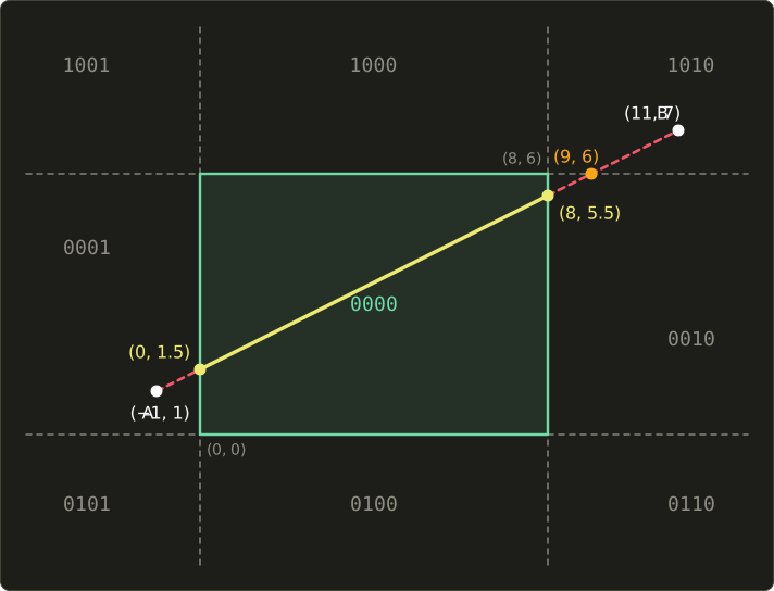
Then for a segment with endpoint codes and :
- If , both endpoints are inside: trivially accept the whole segment.
- If , both endpoints are outside on the same side (both above the top, for example): trivially reject it, the segment can't reach the window.
- Otherwise, take an endpoint that is outside, move it to the intersection with one of the edges its code names, recompute its code, and go back to step 1.
The beauty is that steps 1 and 2 are just bit operations, and in a typical scene most segments are decided there without computing any intersection.
Worked example. Window , segment from to .
The segment's direction is , so its slope is .
- Codes: A is left of the window, . B is above and to the right, .
- OR is 1011, not zero, so no trivial accept. AND is 0000, so no trivial reject.
- A is outside, its code says left. Intersect with : . A becomes with code 0000.
- Still no decision (B is 1010), so clip B. Its code says top first. Intersect with : . B becomes , but its new code is 0010: still right of the window.
- Clip B again, against : . B becomes with code 0000.
- Both codes are 0000: accept –.
The step through shows why the algorithm loops: one intersection may land on another outside region.
Here it is in C++:
enum : int { LEFT = 1, RIGHT = 2, BOTTOM = 4, TOP = 8 };

struct Rect {
  float xmin, ymin, xmax, ymax;
};

int outcode(Vec2 p, const Rect &r) {
  int code = 0;
  if (p.x < r.xmin) code |= LEFT;
  else if (p.x > r.xmax) code |= RIGHT;
  if (p.y < r.ymin) code |= BOTTOM;
  else if (p.y > r.ymax) code |= TOP;
  return code;
}

// Cohen-Sutherland: clips the segment a-b to the rectangle r.
// Returns false when nothing of the segment is left.
bool clipLine(Vec2 &a, Vec2 &b, const Rect &r) {
  int ca = outcode(a, r), cb = outcode(b, r);
  while (true) {
    if ((ca | cb) == 0) return true;  // both inside: accept
    if ((ca & cb) != 0) return false; // both outside on the same side: reject
    int c = ca ? ca : cb;             // pick an endpoint that is outside
    Vec2 p;
    if (c & TOP) {
      p = {a.x + (b.x - a.x) * (r.ymax - a.y) / (b.y - a.y), r.ymax};
    } else if (c & BOTTOM) {
      p = {a.x + (b.x - a.x) * (r.ymin - a.y) / (b.y - a.y), r.ymin};
    } else if (c & RIGHT) {
      p = {r.xmax, a.y + (b.y - a.y) * (r.xmax - a.x) / (b.x - a.x)};
    } else {
      p = {r.xmin, a.y + (b.y - a.y) * (r.xmin - a.x) / (b.x - a.x)};
    }
    if (c == ca) {
      a = p;
      ca = outcode(a, r);
    } else {
      b = p;
      cb = outcode(b, r);
    }
  }
}
With Rect window{0, 0, 8, 6} and the segment above, outcode returns 1 and 10 (0001 and 1010 in binary), and clipLine leaves a at and b at .
A segment from to (both codes 0010) is rejected immediately.
Liang–Barsky, briefly
The Liang–Barsky algorithm (リャン・バースキーのアルゴリズム) writes the segment as with and computes, for each of the four edges, the parameter t where the line crosses it.
With and , the four inequalities "inside the window" all have the form :
| Edge | ||
|---|---|---|
| left | ||
| right | ||
| bottom | ||
| top |
Where the line enters through that edge at , where it leaves.
The visible part runs from the largest entering t (at least 0) to the smallest leaving t (at most 1), and if that interval is empty, nothing is visible.
For our segment, and : entering values (left) and (bottom), leaving values (right) and (top).
So runs from to , which gives and again, with no loop and at most four divisions.
Sutherland–Hodgman polygon clipping
Clipping a polygon is more than clipping its edges one by one, because the result must again be a closed polygon: where the polygon leaves the window and comes back, a piece of the window's border becomes a new edge.
The Sutherland–Hodgman algorithm (サザーランド・ホッジマンのアルゴリズム) does it with a simple trick: clip the whole polygon against one edge (one half-plane) at a time, and feed the result to the next edge.
For one half-plane, walk around the polygon and look at each edge from the previous vertex to the current vertex :
| Output | ||
|---|---|---|
| inside | inside | |
| inside | outside | the intersection |
| outside | outside | nothing |
| outside | inside | the intersection , then |
Worked example. Window again, triangle , , , clipped in the order left, right, bottom, top.
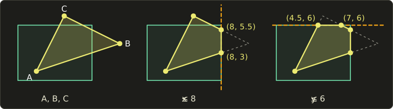
- Left (): all three vertices are inside, the list stays A, B, C.
- Right (): edge C→A is in→in, output A. Edge A→B is in→out: on AB, and , output . Edge B→C is out→in: on BC, and , output and then C. New list: , a quadrilateral.
- Bottom (): everything is inside, nothing changes.
- Top (): edge C→A is out→in, the crossing is at from C, so ; output and then A. Edges A→(8, 3) and (8, 3)→(8, 5.5) are in→in, output and . Edge (8, 5.5)→C is in→out, the crossing is at , so ; output .
Result: the pentagon .
A triangle went in and five vertices came out, which is normal: each window edge can add one vertex.
Sutherland–Hodgman works for any polygon against a convex clipping region; with a concave polygon the result can contain zero-width "bridge" edges along the window border, which a rasterizer draws as nothing but which other algorithms (like Weiler–Atherton) avoid.
Clipping in homogeneous clip space
A GPU clips in clip coordinates, before the perspective division, against the six planes , and (Vulkan: ).
These are still planes in 4D, so Sutherland–Hodgman works unchanged: "inside the left plane" is , "inside the near plane" is , and the intersection parameter is the ratio of these signed values.
Why before the division?
Look at a segment from our vertex P, camera , to a point Q behind the camera at camera :
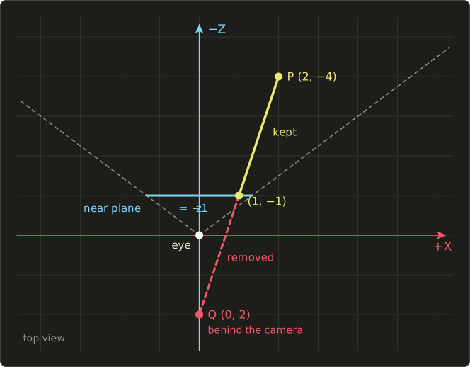
In clip coordinates P is and Q is .
Q has : it's behind the eye.
If we divided first, Q would become , the center of the screen, and the rasterizer would draw a line from P's position towards the center.
But the real segment, seen from the camera, runs away from the center until it leaves the view at the near plane.
Clipping against the near plane does it right.
The signed values are for P and for Q, so the crossing is at
Dividing by gives NDC : depth −1 is exactly the near plane, and the visible segment runs from outwards to .
As a check, the projection matrix is linear, so the same in camera space gives the midpoint of and , which is : on the near plane , as it should be.
After near-plane clipping every remaining vertex has , so the division is always safe.
In practice, many GPUs only clip triangles against the near (and far) plane for real.
For x and y they use a large "guard band" and simply let the rasterizer skip pixels outside the viewport, which is cheaper than creating new vertices.
The result on screen is the same.
6.4 Culling
Clipping cuts primitives.
Culling (カリング) throws whole primitives or objects away before they cost anything.
Back-face culling
In a closed object, like our cube, the faces turned away from the camera are always hidden behind the faces turned towards it.
Back-face culling (背面除去, バックフェースカリング) skips them, which removes roughly half of the triangles of a closed mesh.
A face is a back face when its normal points away from the eye.
With the face normal , a point on the face and the eye :
Note that it's , the direction from the face to the eye, and not one fixed viewing direction: with a perspective camera every face is seen from a slightly different direction.
Worked example in camera space (eye at the origin): the triangle , , has the normal , pointing at the camera.
, a front face.
List the same vertices as A, C, B and the normal flips to , the dot product becomes −20, and it's a back face.
That's why the order of a triangle's vertices (its winding) matters.
GPUs do the test after projection, in screen space: a front face's vertices appear counter-clockwise on screen (OpenGL's default, glFrontFace(GL_CCW)), and the sign of the triangle's signed area decides.
We'll compute that signed area with the edge function in section 6.9.
If your conventions flip y (Vulkan's y-down NDC, for example), the on-screen winding of every triangle flips too, and the front-face setting must match, or the whole model disappears.
Back-face culling is not a complete hidden-surface algorithm: for an object with concave parts or for several objects, front faces can still hide each other, which is the topic of chapter 10.
View-frustum culling
View-frustum culling (視錐台カリング) skips whole objects that can't be visible.
Testing every triangle would be too slow, so each object gets a simple bounding volume (バウンディングボリューム), usually a sphere or a box, and only that is tested against the six planes of the frustum.
For a sphere with center (in camera space) and radius , and one of the four side planes, which pass through the eye, with inward unit normal , the signed distance is (the near and far planes don't pass through the eye, so their distance gets an extra constant, for example for the near plane):
- : completely outside this plane, so cull the object.
- for all six planes: completely inside, no clipping needed at all.
- otherwise the object is drawn, and its triangles are clipped as usual.
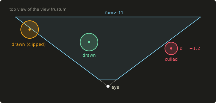
Worked example with the camera of section 6.2 (90° vertical field of view, aspect 4/3).
The half-width of the view at distance is , so the right plane seen from above is , or .
Its inward unit normal is .
A sphere at camera position with radius 1:
It's entirely outside, and none of its (maybe thousands of) triangles reach the GPU.
Game engines go further and organize the bounding volumes in a hierarchy (a bounding volume hierarchy or a scene tree), so a single test can cull a whole building with everything in it.
Exam points
- The order: modeling transform → view transform → projection transform → clipping → perspective division → viewport transform. Clipping comes before the division.
- Clip-space test: inside when . Points behind the camera have .
- Cohen–Sutherland: OR = 0000 → accept, AND ≠ 0000 → reject, otherwise intersect and repeat. AND = 0000 does not mean the segment is visible.
- Sutherland–Hodgman clips against one edge at a time; the output can have more vertices than the input.
- Back-face culling uses the normal (or the winding), and it is not full hidden-surface removal.
6.5 The drawing pipeline on a GPU
Now the machine.
Here are the stages a GPU runs for every draw call, in order:
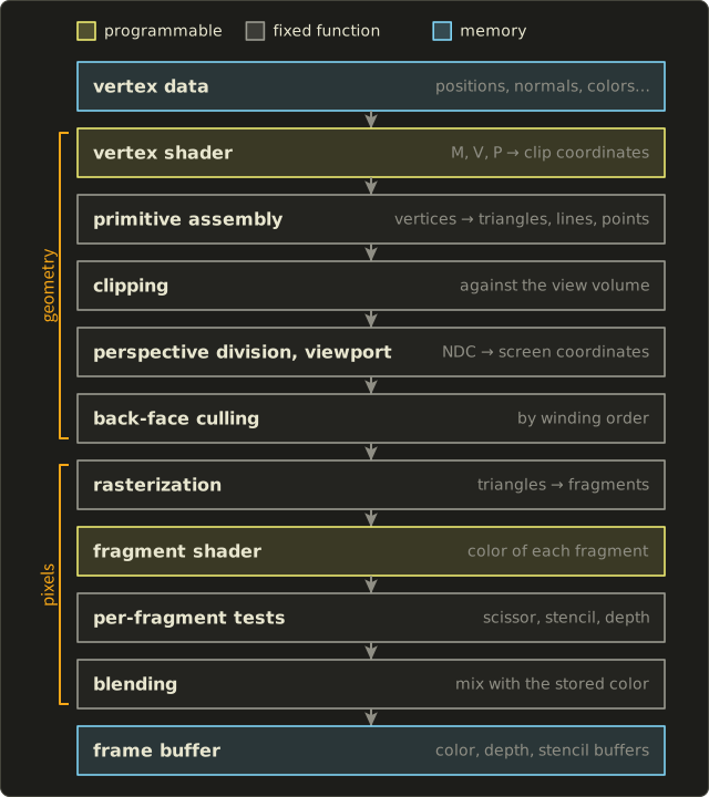
- Vertex data: the positions, normals, colors and texture coordinates of the model, in GPU memory.
- Vertex processing (頂点処理), done by the vertex shader: runs once per vertex and outputs clip coordinates, plus any values to pass on (normals, colors…). Lighting per vertex was also done here in older renderers.
- Primitive assembly (プリミティブアセンブリ): groups vertices into primitives, usually triangles, according to the index list.
- Clipping against the view volume (section 6.3).
- Perspective division and viewport transform (section 6.2).
- Back-face culling by the winding of the screen-space triangle (section 6.4).
- Rasterization (ラスタライズ): finds the pixels each triangle covers and creates a fragment (フラグメント) for each, with interpolated values (sections 6.6 to 6.9).
- Fragment (pixel) processing, done by the fragment shader (pixel shader in Direct3D): computes each fragment's color, with textures and lighting.
- Per-fragment tests: the scissor test (inside a rectangle?), the stencil test (ステンシルテスト, compares with a per-pixel mask) and the depth test (深度テスト, Zテスト: is this fragment in front of what's already stored?). A fragment that fails is discarded.
- Blending (ブレンディング): combines the fragment's color with the color already stored, for transparency (アルファブレンディング).
- Frame buffer (フレームバッファ): the memory that holds the image.
The stages up to the viewport transform are called the geometry stages, the rest the pixel (raster) stages.
Many GPUs move the depth test before the fragment shader when the shader doesn't change the depth ("early-Z"), so hidden fragments aren't even shaded; the result is the same.
The depth test is the z-buffer algorithm, explained in chapter 10.
The frame buffer
The frame buffer is several images of the same size:
- the color buffer: the picture itself, typically 8 bits per channel (RGBA),
- the depth buffer (Z buffer, Zバッファ): one depth value per pixel,
- the stencil buffer: a small integer per pixel, for masks and outlines.
Sizes add up quickly.
A 1920×1080 color buffer with 4 bytes per pixel is bytes, about 7.9 MiB, and a typical 24-bit depth plus 8-bit stencil buffer takes the same again.
Double buffering and v-sync
If the GPU drew directly into the image the monitor is showing, you would see half-finished frames.
Double buffering (ダブルバッファ) uses two color buffers: the front buffer is shown while the GPU draws into the back buffer, and when the frame is finished the two are swapped.
The monitor reads the image line by line from top to bottom, refresh after refresh.
If the swap happens in the middle of that scan, the top of the screen shows the old frame and the bottom the new one, with a visible seam called tearing (テアリング).
V-sync (vertical synchronization, 垂直同期) delays the swap until the monitor has finished a refresh (the vertical blank).
At 60 Hz that leaves ms per frame.
The price: if a frame takes 20 ms, it misses one refresh and is shown after 33.3 ms, so the frame rate drops from 60 straight to 30 with plain double buffering.
Triple buffering (a second back buffer, so the GPU can keep working) and displays with a variable refresh rate soften this.
Fixed function and programmable shaders
In early graphics APIs (OpenGL 1.x, Direct3D up to version 7) every stage was fixed function (固定機能): you could only set parameters, like the light positions or a fog color, and the hardware's built-in formulas did the rest.
In the early 2000s the vertex and pixel stages became programmable (プログラマブルシェーダー): Direct3D 8 (2000) introduced vertex and pixel shaders, and OpenGL 2.0 (2004) brought GLSL.
Modern core APIs (OpenGL's core profile, Vulkan, Direct3D 10 and later) have no fixed-function vertex or pixel stage left at all: you must write at least a vertex shader, and a fragment shader for anything that writes color.
Clipping, rasterization, the tests and blending are still fixed (blending is configurable but not programmable), because they're simple and need to be extremely fast.
Chapter 17 looks at GPUs and real-time systems in more detail, and the GLSL series and OpenGL series let you program these stages yourself.
6.6 Rasterizing lines: DDA and Bresenham
Rasterization, also called scan conversion (スキャン変換 or 走査変換), turns a shape described by coordinates into a set of pixels.
The classic algorithms all answer the same question as cheaply as possible: which pixels are closest to the ideal shape?
A note on coordinates: for the line and circle algorithms I follow the classic convention and treat pixel as the point with integer coordinates , so endpoints sit on pixel centers.
For filling polygons and triangles (sections 6.8 and 6.9) I switch to the GPU convention, where pixel is the square from to with its center at .
In both cases y points up, like graph paper and OpenGL window coordinates.
DDA
Take a line from to with slope between 0 and 1.
Then x changes faster than y, so we draw exactly one pixel per column.
The DDA (digital differential analyzer) steps x by 1 and y by m, and rounds:
For the line from to , , and the y values are 1, 1.4, 1.8, 2.2, 2.6, 3.0, 3.4, 3.8, 4.2, 4.6, 5.0, which round to 1, 1, 2, 2, 3, 3, 3, 4, 4, 5, 5.
It works, but it needs floating point additions and a rounding per pixel, and the repeated addition of 0.4 (not exact in binary) slowly accumulates error on long lines.
Bresenham's line algorithm
Bresenham's algorithm (ブレゼンハムのアルゴリズム) produces the same pixels with integer additions only.
Suppose we have just drawn pixel .
The next column is , and the only two candidates are the pixel straight to the right, E , and the one up and to the right, NE .
The ideal line at that column has height .
Its distances to the two candidates are
and NE is closer exactly when the difference is positive:
The slope is a fraction, so multiply by (positive, so the sign doesn't change) and call the result the decision variable:
Only integers are left.
Even better, we never compute from scratch.
From one column to the next, x grows by 1 and y grows by 0 or 1, so
and the start value, using the fact that the first pixel lies exactly on the line, is
The whole algorithm:
- if : go to NE ( + 1) and add ,
- if : go to E and add .
(When the line passes exactly halfway between the two pixels, and either choice is fine; I take NE.)
Worked trace for to : , , so , the E step adds 8 and the NE step adds −12.
| x | y | decision | |
|---|---|---|---|
| 1 | 1 | −2 | E: −2 + 8 = 6 |
| 2 | 1 | 6 | NE: 6 − 12 = −6 |
| 3 | 2 | −6 | E: −6 + 8 = 2 |
| 4 | 2 | 2 | NE: 2 − 12 = −10 |
| 5 | 3 | −10 | E: −10 + 8 = −2 |
| 6 | 3 | −2 | E: −2 + 8 = 6 |
| 7 | 3 | 6 | NE: 6 − 12 = −6 |
| 8 | 4 | −6 | E: −6 + 8 = 2 |
| 9 | 4 | 2 | NE: 2 − 12 = −10 |
| 10 | 5 | −10 | E: −10 + 8 = −2 |
| 11 | 5 | −2 | (end) |
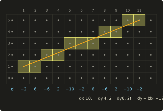
The pixels are identical to the DDA's, and the last pixel ends exactly at , because the integer arithmetic has no rounding error to accumulate.
#include <cstdio>

// Bresenham's line algorithm for 0 <= dy <= dx (slope between 0 and 1).
// plot(x, y) sets one pixel.
template <class Plot>
void bresenham(int x0, int y0, int x1, int y1, Plot plot) {
  int dx = x1 - x0, dy = y1 - y0;
  int d = 2 * dy - dx; // the decision variable
  int y = y0;
  for (int x = x0; x <= x1; ++x) {
    plot(x, y);
    if (d >= 0) {
      ++y; // the upper pixel (NE) was closer
      d += 2 * (dy - dx);
    } else {
      d += 2 * dy; // the lower pixel (E) was closer
    }
  }
}

int main() {
  bresenham(1, 1, 11, 5, [](int x, int y) { printf("(%d, %d) ", x, y); });
  printf("\n");
  return 0;
}
(1, 1) (2, 1) (3, 2) (4, 2) (5, 3) (6, 3) (7, 3) (8, 4) (9, 4) (10, 5) (11, 5) The other seven octants reuse the same code by symmetry: if (a steep line) swap the roles of x and y and step along y; if the line goes to the left, swap the two endpoints; if it goes down, step y by −1 instead of +1.
6.7 The midpoint circle algorithm
A circle has 8-fold symmetry: if is on a circle around the origin, so are and .
So we only compute one eighth, the arc from going right until , where the slope is between 0 and −1, and mirror every pixel into the other seven octants.
On this arc x always grows by 1 and y either stays or drops by 1.
The midpoint algorithm (中点アルゴリズム) decides by testing the point halfway between the two candidates, , with the circle function
which is negative inside the circle and positive outside.
If the midpoint is inside (), the circle passes above it and we keep y; otherwise we step down.
Writing and expanding the squares gives integer updates:
- if : keep y, and ,
- else: , and ,
with , which we round to (all the updates are integers and only the sign of p matters, so the quarter never changes a decision).
Worked trace for , :
| x | y | next | |
|---|---|---|---|
| 0 | 8 | −7 | keep y: −7 + 2 · 1 + 1 = −4 |
| 1 | 8 | −4 | keep y: −4 + 2 · 2 + 1 = 1 |
| 2 | 8 | 1 | step down: 1 + 2 · 3 + 1 − 2 · 7 = −6 |
| 3 | 7 | −6 | keep y: −6 + 2 · 4 + 1 = 3 |
| 4 | 7 | 3 | step down: 3 + 2 · 5 + 1 − 2 · 6 = 2 |
| 5 | 6 | 2 | next would be (6, 5): past x = y, stop |
Check one of them against the true circle: at the exact height is , which rounds to 7, the pixel we chose.
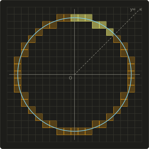
The yellow pixels are the six we computed; the orange ones are their mirror images.
6.8 Filling polygons with scanlines
To fill a polygon we could test every pixel against it, but there's a smarter classic: the scanline algorithm (スキャンライン法).
Process the image one row (scanline) at a time, at the height of the pixel centers, .
On each scanline, find where the polygon's edges cross it, sort these x values, and fill between them in pairs: from the 1st to the 2nd crossing, from the 3rd to the 4th, and so on.
That's the even-odd (parity) rule (偶奇規則): a point is inside when a ray from it to the right crosses the boundary an odd number of times.
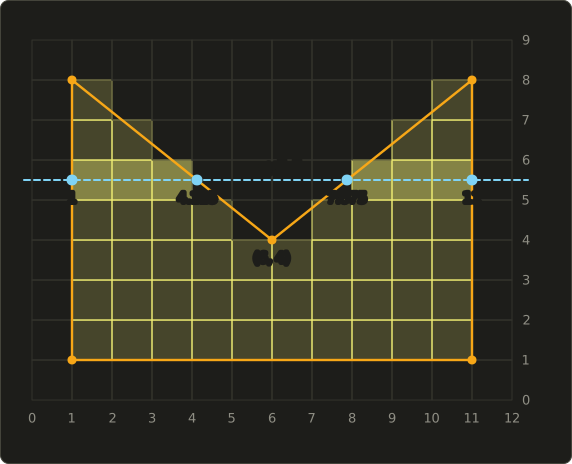
Worked example. The polygon has a V-shaped notch at the top.
The scanline crosses four edges:
- the left edge and the right edge ,
- the edge from to : x drops by per unit of y, so ,
- the edge from to : .
Sorted: 1, 4.125, 7.875, 11.
Fill the pairs and : the pixel centers 1.5, 2.5, 3.5 are in the first span and 8.5, 9.5, 10.5 in the second, so this row gets pixels 1, 2, 3 and 8, 9, 10.
Pixels 4 to 7 (centers 4.5 to 7.5) fall into the notch.
Edge table and active edge list
Computing every crossing from scratch is wasteful.
The classic implementation keeps two lists:
- The edge table (エッジテーブル, 辺リスト): every non-horizontal edge, sorted by its lower end , with , the x at , and . Horizontal edges are dropped: they never cross a scanline.
- The active edge list (アクティブエッジリスト): the edges that cross the current scanline, each with its current x.
For each scanline: move the edges that start here from the edge table into the active list, remove the edges that have ended, sort by x, fill the pairs, then add to every x for the next scanline.
In our example the two slanted edges become active at with and and .
Their crossings move outwards by 1.25 per scanline: 5.375 and 6.625 at , 4.125 and 7.875 at , 2.875 and 9.125 at , and 1.625 and 10.375 at .
Counting all rows gives 50 pixels, exactly the polygon's area (the shoelace formula gives 50 too); in general the count is only close to the area, not equal.
Vertices on a scanline
What if a scanline passes exactly through a vertex?
Then two edges meet there, and counting the crossing twice or once must be done right, or parity breaks.
The standard rule makes each edge half-open: an edge counts on scanline y when .
At a vertex where one edge comes up and the other continues up, exactly one of them counts: parity flips once, correct.
At a peak (both edges below the vertex) neither counts, and at a valley (both edges above) both count: parity doesn't change, also correct, because the scanline just touches the polygon there.
Sampling at pixel centers () with integer vertices avoids the case anyway, but the rule is still needed for arbitrary vertices.
Even-odd versus nonzero
For simple polygons both rules agree, but for a self-intersecting polygon like a star drawn in one stroke they don't.
The nonzero winding rule (非ゼロ回転数規則) counts each crossing as +1 or −1 depending on the edge's direction, and a point is inside when the total is not zero.
In the star's center the boundary winds around twice, so the even-odd rule leaves a hole there while the nonzero rule fills it:
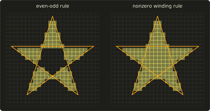
Both images were computed by testing every pixel center with a ray to the right.
Vector formats let you choose: SVG and PDF have a fill-rule setting with exactly these two options.
A completely different family, seed fill (シードフィル), starts from one pixel inside an already drawn outline and spreads to its neighbors, like a paint program's bucket tool; it fills by pixels, not by geometry.
6.9 Triangle rasterization with edge functions
GPUs only rasterize triangles, and they don't use scanlines with sorted lists.
They use edge functions (エッジ関数), because the test is the same simple formula for every pixel, which suits thousands of parallel units.
The edge function
For a directed edge from to and a point :
This is the z component of the cross product (Linear Algebra chapter 5), so it's positive when is to the left of the edge, negative to the right, and zero on the line.
For a triangle A, B, C listed counter-clockwise (with y up), the inside is to the left of all three edges:
The rasterizer loops over the pixels of the triangle's bounding box and tests each pixel center.
Moving one pixel to the right changes by the constant , so after the first pixel each test costs three additions.
And is twice the triangle's signed area: positive for counter-clockwise, negative for clockwise.
That's the back-face test of section 6.4.
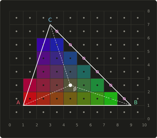
Worked example. Triangle , , .
: counter-clockwise, front-facing, area 24.
Test the pixel center :
All positive, so the pixel is covered.
The center instead gives : outside, to the right of BC.
The top-left rule
Look at the pink circles in the picture: those pixel centers lie exactly on the edge BC, where .
If another triangle shares that edge (two triangles of a quad, for example), both would claim those pixels with a "≥ 0" test, the pixel would be drawn twice (wrong with transparency), and with "> 0" in both it would be drawn by neither (a crack).
So the rasterization rules of real APIs require that a pixel center on a shared edge belongs to exactly one of the two triangles; OpenGL's specification, for example, states exactly this.
Direct3D defines the specific tie-break as the top-left rule (トップレフトルール): a center exactly on an edge is covered only if that edge is a top edge (exactly horizontal, with the triangle below it) or a left edge (on the left side of the triangle).
For a counter-clockwise triangle with y up, a left edge is one that goes down ().
In our triangle CA goes down, so the centers and on CA are covered, while BC goes up, so the six centers on BC are left to the neighbor.
That gives the 22 colored pixels in the picture.
Barycentric interpolation
Rasterization must also give each fragment values from the vertices: colors, texture coordinates, depth.
The three edge functions give them for free.
Divide them by the whole :
These are the barycentric coordinates (重心座標) of : each one is the area of the small triangle opposite a vertex, divided by the whole area (the dashed lines in the picture split the triangle into these three parts).
They are never negative inside the triangle, they add up to 1, and exactly at A.
Any vertex value is then interpolated as
For our pixel: , , , and .
With A red , B green and C blue , the pixel's color is , an olive brown, which is exactly the color of that cell in the picture.
The same weights interpolate the depth for the depth test.
Here is the rasterizer, with the top-left rule, printing the covered pixels (top row first) and the weights of our pixel:
#include <cstdio>
#include "linalg.hh"

// Edge function: positive when p is to the left of the directed edge a -> b (y up).
float edgeFunction(Vec2 a, Vec2 b, Vec2 p) {
  return (b.x - a.x) * (p.y - a.y) - (b.y - a.y) * (p.x - a.x);
}

// Top-left rule for a counter-clockwise triangle with y up:
// a left edge goes down, a top edge is horizontal and goes left.
bool isTopLeft(Vec2 a, Vec2 b) {
  return b.y < a.y || (b.y == a.y && b.x < a.x);
}

bool covers(float e, Vec2 a, Vec2 b) {
  return e > 0 || (e == 0 && isTopLeft(a, b));
}

int main() {
  Vec2 a{1, 1}, b{9, 1}, c{3, 7}; // counter-clockwise, y up
  float area2 = edgeFunction(a, b, c); // twice the area
  const int width = 10, height = 8;
  for (int y = height - 1; y >= 0; --y) { // print the top row first
    for (int x = 0; x < width; ++x) {
      Vec2 p{x + 0.5f, y + 0.5f}; // the pixel center
      float e0 = edgeFunction(b, c, p), e1 = edgeFunction(c, a, p), e2 = edgeFunction(a, b, p);
      bool in = covers(e0, b, c) && covers(e1, c, a) && covers(e2, a, b);
      putchar(in ? '#' : '.');
    }
    putchar('\n');
  }
  // barycentric coordinates of one pixel center
  Vec2 p{4.5f, 2.5f};
  float la = edgeFunction(b, c, p) / area2;
  float lb = edgeFunction(c, a, p) / area2;
  float lc = edgeFunction(a, b, p) / area2;
  printf("lambda = (%g, %g, %g)\n", la, lb, lc);
  return 0;
}
..........
..........
..##......
..###.....
..####....
.######...
.#######..
..........
lambda = (0.375, 0.375, 0.25)
Perspective-correct interpolation
One catch: the weights above are measured on the screen.
Under perspective projection, equal steps on the screen are not equal steps on the 3D triangle (the far part is squeezed), so interpolating texture coordinates with screen-space weights makes textures wobble and bend.
The fix, perspective-correct interpolation (パースペクティブコレクト補間), interpolates and linearly on the screen and divides the two per pixel.
GPUs do this automatically for every varying.
NDC depth is the exception: it is an affine function of the screen position, so it can be interpolated linearly as it is, which is part of why the z-buffer works so well.
Part 2 derives all of this.
Anti-aliasing in the pipeline
Testing only the pixel center is point sampling, so triangle edges get the jaggies we met in chapter 2.
The fix is to sample more: supersampling tests several points per pixel and shades each one, while MSAA (multisample anti-aliasing) tests coverage at several points but runs the fragment shader once per pixel.
Part 2 covers these, and you'll switch MSAA on yourself in the OpenGL series.
Exam points
- Bresenham uses only integer additions; the decision variable starts at and grows by (E) or (NE). DDA needs floating point and rounding.
- The midpoint circle algorithm computes one octant and mirrors it 8 ways.
- Scanline filling: crossings sorted by x, filled in pairs (even-odd rule); edges are half-open in y; horizontal edges are skipped.
- Even-odd and nonzero only differ for self-intersecting polygons.
- Edge functions: inside when all three have the same sign; their ratios are the barycentric coordinates, which add up to 1.
6.10 Summary
- The viewing pipeline: object → (modeling transform) → world → (view transform) → camera → (projection transform) → clip → clipping → (perspective division) → NDC → (viewport transform) → screen.
- Clipping happens in clip space, , before the division, because points behind the camera have .
- Cohen–Sutherland uses 4-bit outcodes for quick accepts (OR = 0) and rejects (AND ≠ 0); Liang–Barsky uses the line parameter t; Sutherland–Hodgman clips polygons one window edge at a time.
- Back-face culling drops faces whose normal points away from the eye (decided by winding on screen); view-frustum culling drops objects whose bounding volume is outside a frustum plane.
- The GPU drawing pipeline: vertex shader, primitive assembly, clipping, division and viewport, culling, rasterization, fragment shader, tests (scissor, stencil, depth), blending, frame buffer.
- Double buffering hides unfinished frames; v-sync swaps during the vertical blank to prevent tearing.
- DDA steps by the slope with rounding; Bresenham decides between E and NE with an integer decision variable; the midpoint circle algorithm does the same for one octant of a circle.
- Scanline filling sorts edge crossings and fills pairs; GPUs test pixel centers with edge functions, use the top-left rule on shared edges, and interpolate with barycentric coordinates.
6.11 Key terms
| English | 日本語 |
|---|---|
| viewing pipeline | ビューイングパイプライン |
| drawing (rendering) pipeline | 描画パイプライン |
| modeling transform | モデリング変換 |
| view transform | ビュー変換(視野変換) |
| projection transform | 投影変換 |
| camera (view) coordinates | カメラ座標系(視点座標系) |
| clip coordinates | クリップ座標系 |
| perspective division | 透視除算 |
| normalized device coordinates (NDC) | 正規化デバイス座標系 |
| viewport transform | ビューポート変換 |
| screen (device) coordinates | スクリーン座標系(デバイス座標系) |
| clipping | クリッピング |
| outcode | 領域コード(アウトコード) |
| culling | カリング |
| back-face culling | 背面除去(バックフェースカリング) |
| view-frustum culling | 視錐台カリング |
| bounding volume | バウンディングボリューム |
| vertex processing | 頂点処理 |
| primitive assembly | プリミティブアセンブリ |
| rasterization, scan conversion | ラスタライズ、スキャン変換 |
| fragment | フラグメント |
| depth test | 深度テスト(Zテスト) |
| stencil test | ステンシルテスト |
| blending | ブレンディング |
| frame buffer | フレームバッファ |
| double buffering | ダブルバッファ |
| vertical sync (v-sync) | 垂直同期 |
| tearing | テアリング |
| fixed function | 固定機能 |
| programmable shader | プログラマブルシェーダー |
| Bresenham's algorithm | ブレゼンハムのアルゴリズム |
| midpoint algorithm | 中点アルゴリズム |
| scanline algorithm | スキャンライン法 |
| edge table, active edge list | エッジテーブル、アクティブエッジリスト |
| even-odd rule | 偶奇規則 |
| nonzero winding rule | 非ゼロ回転数規則 |
| edge function | エッジ関数 |
| top-left rule | トップレフトルール |
| barycentric coordinates | 重心座標 |
| perspective-correct interpolation | パースペクティブコレクト補間 |
6.12 Challenges
- ★ Follow the object-space vertex through the pipeline of section 6.2 (same M, V, P and 800×600 window): world, camera and clip coordinates, the clip test, NDC, the pixel and the depth buffer value. (Check: the camera z must lie between −1 and −11.)
- ★ With the window , give the outcodes of and and clip the segment between them with Cohen–Sutherland, writing down every intermediate point and code. Then show with outcodes alone that the segment from to is invisible.
- ★★ Clip the triangle , , against the window with Sutherland–Hodgman in the order left, right, bottom, top, and write the vertex list after each step. How many vertices does the result have?
- ★★ For the triangle , , (y up), decide with edge functions whether the pixel center is inside, compute its barycentric coordinates, and interpolate the depth if A, B and C have depths 0.2, 0.8 and 0.5. Then list the vertices as A, C, B: what happens to the signs, and what does that mean for back-face culling?
- ★★★ A segment in camera space goes from to and is projected with . Show that its endpoints land at and , then find which 3D point lands at the screen midpoint . What fraction of the way along the 3D segment is it, and what does that tell you about interpolating texture coordinates with screen-space weights?
Multiple choice
Q1 ★ Which of the following lists the stages of the viewing pipeline in the correct order?
| A | modeling transform → view transform → clipping → viewport transform → projection transform → perspective division |
| B | modeling transform → projection transform → view transform → clipping → perspective division → viewport transform |
| C | modeling transform → view transform → projection transform → perspective division → clipping → viewport transform |
| D | view transform → modeling transform → projection transform → clipping → viewport transform → perspective division |
| E | modeling transform → view transform → projection transform → clipping → perspective division → viewport transform |
Q2 ★ In Cohen–Sutherland line clipping, each endpoint of a segment gets a 4-bit outcode. Which of the following statements is correct?
| A | If the bitwise OR of the two codes is not 0000, the whole segment is outside the window. |
| B | If the bitwise AND of the two codes is 0000, at least part of the segment is always inside the window. |
| C | The outcode has one bit for each of the nine regions around the window. |
| D | If the bitwise AND of the two codes is not 0000, the whole segment is outside the window and can be rejected without computing any intersection. |
| E | If one endpoint has the code 0000, the segment never needs to be clipped. |
Q3 ★★ A line from to is drawn with Bresenham's algorithm (step to the upper pixel when the decision variable is 0 or more). Which pair gives the initial decision variable and the second pixel drawn?
| A | , second pixel |
| B | , second pixel |
| C | , second pixel |
| D | , second pixel |
| E | , second pixel |
6.13 Practical assignment
Take one triangle through the whole chapter on graph paper: projection, clipping, culling, filling, a Bresenham edge and interpolation.
You need a sheet of graph paper with at least a 20×16 grid, a ruler, a pencil, two colored pens and a calculator.
The camera-space vertices are , and .
The projection is the OpenGL perspective matrix with a 90° vertical field of view, aspect ratio 1, and (so its entries are 1, 1, −1.25, −2.25 and −1), and the window is 16×16 pixels with the origin at the bottom-left and y up: , .
- Project. Compute the clip coordinates of A, B and C and apply the clip test to each. Which vertex is outside, and against which plane?
- Divide and map. Compute NDC and window coordinates for all three vertices (including the outside one; its w is positive, so the division is safe). Write down the three NDC depths too.
- Cull. Compute in window coordinates. Is the triangle counter-clockwise, so front-facing with OpenGL's default?
- Clip. Draw the 16×16 window and the whole triangle on the graph paper (the triangle sticks out on one side). Because all three w values are positive, clipping the projected triangle against the window edge gives the same polygon as clipping in clip space. Clip it with Sutherland–Hodgman and write down the resulting polygon.
- Fill. For each scanline , compute the crossings with the clipped polygon's edges and shade the pixels whose centers lie between the pairs (even-odd rule). Count the shaded pixels and compute the polygon's area with the shoelace formula; the two numbers should be close.
- Draw an edge. With the second pen, draw the edge from A to C with Bresenham's algorithm. It is steep, so swap the roles of x and y: step y by 1 and decide whether x stays or moves right. Write down every decision value, and compare the pixels with the left border of your filled region.
- Interpolate. For the pixel , center , compute the barycentric coordinates with respect to the unclipped triangle ABC in window coordinates. Give A red, B green and C blue and compute the pixel's color, then interpolate the NDC depth and convert it to a depth buffer value .
How to check yourself: every vertex of the clipped polygon lies inside the window or on its border; the barycentric coordinates are all positive and add up to exactly 1; the interpolated depth lies between the smallest and largest vertex depths; and the pixel count from step 5 differs from the area by only a few pixels.
For an extra check of step 4, find where the edge AB meets the plane in clip space (the parameter t where changes sign), divide that point by its w, and confirm that it lands on the same window position as your screen-space clip, even though the t values on the screen and in clip space are different.
コメント(0)
まだコメントはありません。
ログインするとコメント出来ます。