14. Animation 2: Physics, Procedural Animation and Compositing
In chapter 13 an animator decided every motion: keyframes, curves, skeletons, a captured performance.
That works for a character, but nobody wants to keyframe ten thousand sparks, a flag in the wind, a glass shattering or a flock of three hundred birds.
For those, we let the computer compute the motion: from the laws of physics, or from simple rules that we write down once.
And when the finished CG has to sit inside a real film shot, it has to move with the real camera and blend with the real pixels.
This chapter covers four syllabus items of area 5 (animation): physics-based animation (物理ベースアニメーション), real-time animation (リアルタイムアニメーション), procedural animation (手続き型アニメーション) and compositing with live action (実写映像との合成).
That means numerical integration and its stability, particle systems, mass–spring systems, rigid bodies, collisions and fluids; frame budgets, game loops and animation blending; noise, flocking (boids) and crowds; and matchmoving, chroma key, alpha mattes, rotoscoping and lighting matches.
Keyframes, skeletons, skinning and motion capture are in chapter 13; image filtering and editing in general are chapter 15; GPUs and the hardware side of real-time systems are chapter 17.
The math we need is vectors, lengths and the dot product (Linear Algebra chapters 2 to 4), the cross product (Linear Algebra chapter 5) and a little school physics: velocity, acceleration and Newton's second law, which I'll recap.
14.1 Physics-based animation
Why simulate
Keyframing one bouncing ball is easy; keyframing fifty balls bouncing off each other with the right heights and timing is not.
Physics-based animation (物理ベースアニメーション) gives the objects physical properties (mass, stiffness, friction) and lets a simulation (シミュレーション) compute how they move under forces.
The result is physically plausible automatically, and it scales to millions of objects.
The price is control.
A director says "the debris should land just left of the hero, two seconds from now", and physics doesn't take orders.
So production work mixes the two: an animator keyframes the main action, a simulation adds the secondary motion (cloth, hair, debris, splashes), and artists steer the simulation with extra forces, fields and constraints.
State, forces and Newton's second law
For a point mass, everything a simulator needs to know at time is its state (状態): the position and the velocity .
The velocity is the rate of change of the position, and the acceleration is the rate of change of the velocity.
Newton's second law (ニュートンの運動の第2法則) connects the acceleration to the total force acting on a body of mass :
Written as a rule for the state, this is the equation of motion (運動方程式):
The force can depend on where the body is, how fast it moves and when.
The forces that appear again and again in animation:
- Gravity (重力): with m/s² (y up).
- Spring force (バネの力): for a spring stretched by (section 14.4).
- Damping or drag (減衰、空気抵抗): , against the motion.
- Force fields (力場) such as wind, vortices or noise, and contact forces from collisions (section 14.6).
Simulation means: start from a known state, and repeatedly compute the forces and advance the state by a small time step (時間刻み) , for example s.
A ball dropped from height has the exact solution , but as soon as several forces interact there is no formula, and we must step forward numerically.
14.2 Numerical integration
Explicit Euler
The simplest rule assumes that the velocity and acceleration stay constant during one step.
This is the explicit Euler method (陽的オイラー法, also 前進オイラー法 or just オイラー法):
Both updates use only the old state (index ), which is what "explicit" means.
Worked example: a falling ball.
Drop a ball from m with , m/s² and s.
The acceleration is always , so .
- Step 1: , .
- Step 2: , .
- Step 3: , .
The exact height at s is m, so Euler is 0.147 m too high: it always uses the velocity from the start of the step, which is too slow for a ball that keeps speeding up.
The error after a fixed time is proportional to : halve the step and the error halves.
That makes Euler a first-order method (1次精度).
Semi-implicit (symplectic) Euler
Swap the order: update the velocity first, then move with the new velocity:
This is the semi-implicit Euler method (半陰的オイラー法), also called symplectic Euler (シンプレクティックオイラー法).
It costs exactly the same as explicit Euler.
For the falling ball: , ; , ; , .
Now it's 0.147 m too low, because it uses the velocity from the end of each step.
Still first order, so for a falling ball neither is better.
The difference shows up with springs, a little further down.
Verlet integration
The Verlet method (ベルレ法), named after Loup Verlet, who used it for molecular dynamics in 1967, doesn't store the velocity at all.
It computes the next position from the last two:
The velocity is hidden in the difference .
To start, we need , for example from .
For the falling ball: , then
These are exactly the true heights at 0.1, 0.2 and 0.3 s.
Verlet is second order (error proportional to ) and exact for a constant acceleration.
It's popular in games for cloth and ropes: to satisfy a constraint (a rope segment must keep its length) you simply move the positions, and the velocity follows automatically.
Runge–Kutta methods
The Runge–Kutta methods (ルンゲ=クッタ法) improve accuracy by sampling the slope at several points inside the step.
Write the whole state as and its rate of change as .
The midpoint method (RK2) takes a half Euler step to estimate the state in the middle of the step, and then uses the slope there for the full step:
The classic fourth-order Runge–Kutta method (RK4) evaluates four slopes and averages them with the weights 1, 2, 2, 1:
Its error is proportional to : halving the step divides the error by 16.
The cost is four force evaluations per step instead of one, which matters when a force evaluation means computing all collisions of a scene.
| Method | Force evaluations per step | Order (error ∝) | Typical use |
|---|---|---|---|
| explicit Euler | 1 | teaching; rarely in production | |
| semi-implicit Euler | 1 | game physics engines, particles | |
| Verlet | 1 | cloth, ropes, molecular dynamics | |
| RK2 (midpoint) | 2 | smooth forces, offline | |
| RK4 | 4 | accurate smooth motion (orbits, cameras) | |
| implicit Euler | 1 plus solving a system | stiff cloth and soft bodies |
Stability: the spring that explodes
Accuracy is one problem; stability (安定性) is a worse one.
Take a mass kg on a spring with stiffness N/m, pulled to m and released ().
The exact motion is : it oscillates forever between −1 and 1 with the period s, and its energy (エネルギー)
stays at J.
The acceleration is .
With s, explicit Euler gives:
| Step | |||
|---|---|---|---|
| 0 | 1 | 0 | 0.5 |
| 1 | 0.505 | ||
| 2 | 0.51005 | ||
| 3 | 0.5151505 |
The energy grows by exactly 1% per step.
That's no accident.
With , one step maps to , and
so every step multiplies the energy by , here .
After 200 steps (20 s) the energy is times as large, and the amplitude times as large.
For any step size, explicit Euler pumps energy into an undamped oscillator: it is unconditionally unstable for it.
The semi-implicit version with the same gives for the first three steps, and its energy only wobbles between about 0.476 and 0.526 forever:
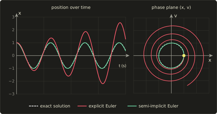
The right half is the phase plane (位相平面): position against velocity.
The exact motion is the unit circle (energy constant); explicit Euler spirals outward, semi-implicit Euler stays on a closed loop.
That property, keeping the energy bounded over very long runs, is what "symplectic" means in practice, and it's the reason almost every game physics engine uses semi-implicit Euler.
It isn't magic, though.
Semi-implicit Euler is stable only while , that is
with the period : about a third of a period.
A stiff (硬い) spring has a large and needs a tiny step.
With N/m and kg, rad/s: at s, , and semi-implicit Euler is fine, while explicit Euler multiplies the energy by every step, so after 10 steps (1 s) it's times as large and the amplitude 32 times.
At s, , and semi-implicit Euler explodes too: goes 1, −5.25, 21.3, −85.3, …
There are three ways out:
- Smaller steps (or several substeps per frame), so that stays small.
- Implicit integration (陰的積分): the implicit Euler method (陰的オイラー法) uses the forces at the end of the step, , so each step means solving a system of equations, but it is stable for any step size. It damps artificially: for our spring the energy is multiplied by per step (after 20 s at only 14% is left), which is acceptable for cloth (Baraff and Witkin, "Large Steps in Cloth Simulation", 1998).
- Damping, physical or artificial, to remove the energy that the integrator adds.
Damping
A damping force turns the endless oscillation into a decaying one.
For a spring, the special value is critical damping (臨界減衰): the mass returns to rest as fast as possible without overshooting.
For , that's .
Less damping leaves a decaying wobble (jelly, a tail, an antenna that lags behind and settles); more creeps back slowly, like a door closer.
Code: explicit vs semi-implicit Euler
This program runs the spring of the table with both methods and prints the position and the energy (no linalg.hh needed for one dimension):
#include <cmath>
#include <cstdio>

// A mass on a spring: m x'' = -k x. The state is the position x and the velocity v.
struct State {
  double x, v;
};

const double m = 1.0, k = 1.0;

double energy(State s) { return 0.5 * m * s.v * s.v + 0.5 * k * s.x * s.x; }

State explicitEuler(State s, double h) {
  double a = -k / m * s.x;               // acceleration from the OLD position
  return {s.x + h * s.v, s.v + h * a};   // both updates use the old state
}

State semiImplicitEuler(State s, double h) {
  double v = s.v + h * (-k / m * s.x);   // velocity first
  return {s.x + h * v, v};               // then position, with the NEW velocity
}

int main() {
  const double h = 0.1;
  State e{1.0, 0.0}, si{1.0, 0.0};
  printf("%4s  %10s  %8s  %10s  %8s\n", "step", "explicit x", "E", "semi x", "E");
  for (int n = 0; n <= 200; ++n) {
    if (n <= 3 || n % 50 == 0) {
      printf("%4d  %10.6f  %8.5f  %10.6f  %8.5f\n", n, e.x, energy(e), si.x, energy(si));
    }
    e = explicitEuler(e, h);
    si = semiImplicitEuler(si, h);
  }
  printf("exact x(20) = cos(20) = %.6f, E = 0.5\n", std::cos(20.0));
  return 0;
}
step  explicit x         E      semi x         E
   0    1.000000   0.50000    1.000000   0.50000
   1    1.000000   0.50500    0.990000   0.49505
   2    0.990000   0.51005    0.970100   0.49035
   3    0.970000   0.51515    0.940499   0.48608
  50    0.343355   0.82232    0.333638   0.51601
 100   -1.408847   1.35241   -0.809385   0.47781
 150   -1.532160   2.22421   -0.796058   0.52573
 200    1.264886   3.65801    0.354578   0.48373
exact x(20) = cos(20) = 0.408082, E = 0.5
The semi-implicit energy stays near 0.5, but its position at 20 s (0.355) is not the exact 0.408: its loop in the phase plane is a slightly tilted ellipse, traversed a little too fast, so it drifts in phase (位相).
RK4 with the same step gives 0.408097 and an energy of 0.4999986, at four times the cost.
14.3 Particle systems in motion
Chapter 9, section 9.5 introduced the particle system (パーティクルシステム) of Reeves (1983) as a way to represent fuzzy shapes like fire and smoke, and promised the motion for this chapter.
A particle is a point mass with a state plus attributes: position, velocity, age, lifetime, color, size, opacity.
Every frame, the system runs the same loop:
- Emit (放出): the emitter (エミッタ) creates new particles at a rate (particles per second) in a region (point, line, surface, volume), with random variation around a mean velocity.
- Apply forces: gravity, drag, wind, attractors, and force fields such as a noise field that makes smoke swirl (the noise of chapter 11).
- Integrate, usually with semi-implicit Euler, and collide with simple shapes (section 14.6).
- Age: change color, size and opacity with age (a spark cools from white to dark red and fades), and remove particles whose lifetime is over.
- Render: usually as small camera-facing textured quads (sprites, billboards), often with additive blending so the order doesn't matter (chapter 10, section 10.12), or as streaks for motion blur.
Worked example: one spark.
A spark is emitted at m with velocity m/s and lifetime 1.5 s, under gravity only.
Its exact path is
It is highest when the vertical velocity is zero, at s, where m and m.
At s it dies at , still in the air: it would only reach the ground at s.
An emitter of 200 sparks per second with this lifetime keeps sparks alive.
Particles that don't interact can all be updated independently, so GPUs simulate millions of them in compute shaders (you'll meet compute shaders in the GLSL series, chapter 15).
Once particles do interact, through springs, collisions or pressure, we get the systems of the next sections.
14.4 Mass–spring systems: cloth, soft bodies and hair
Hooke's law in 3D
Connect particles with springs and you get a mass–spring system (バネ質点系).
A spring between the particles at and with rest length (自然長) and stiffness pulls them together when stretched and pushes them apart when compressed, by Hooke's law (フックの法則):
is the unit vector from A to B (Linear Algebra chapter 3).
To stop the spring from ringing forever, a spring damper adds a force along the spring that resists the relative velocity:
Worked example.
A is at , B at , the rest length is and N/m.
, , : the spring is stretched by 1 m.
Both are pulled toward each other with 50 N.
If B moves away from A with the relative velocity m/s and , the speed of stretching is m/s, and the damper adds to A's force, for a total of .
Cloth
A piece of cloth is a grid of particles with three kinds of springs:
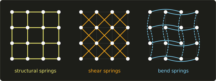
- Structural springs (構造バネ) between direct neighbors resist stretching.
- Shear springs (せん断バネ) along the diagonals resist the square cells collapsing into diamonds.
- Bend springs (曲げバネ) between particles two apart resist folding; weak bend springs give silk, strong ones give leather.
Cloth is where stability bites.
Real fabric barely stretches, so the structural springs must be very stiff.
For a single 10 g particle on a spring of N/m, rad/s and semi-implicit Euler needs s, which a 60 Hz step of 0.0167 s satisfies.
Make the spring ten times stiffer () and rad/s, s: two substeps per frame.
Film cloth therefore uses implicit integration, and games often use position-based dynamics (PBD): instead of stiff springs, they directly move particles back to satisfy distance constraints after each step, the Verlet idea of section 14.2.
The cloth must also collide with the body and with itself (self-collision), which is usually the most expensive part.
Soft bodies and hair
- Soft bodies (ソフトボディ, 弾性体): fill a volume with particles connected by springs (or use a tetrahedral mesh with the finite element method, FEM, 有限要素法). Jelly, fat and muscle jiggle, cushions that compress.
- Hair (髪の毛、ヘア): each strand is a chain of particles with stretch springs and bend springs (plus twist for curly hair). A human head has around 100,000 hairs, so simulators move a few hundred guide hairs and interpolate the rest between them; fur works the same way.
Together with cloth these are deformable bodies (変形体): their shape changes.
The opposite is the rigid body.
14.5 Rigid bodies
A rigid body (剛体) never changes shape: a die, a crate, a car body, a brick.
Its state needs more than a position:
- Linear motion: the position of the center of mass (重心) and its velocity , with exactly as for a particle. A force accelerates the center of mass the same way wherever on the body it acts.
- Angular motion: the orientation (姿勢), stored as a quaternion (Linear Algebra chapter 13) or a rotation matrix, and the angular velocity (角速度) , whose direction is the rotation axis and whose length is the speed in rad/s.
A force applied at an offset from the center of mass also creates a torque (トルク), with the cross product of Linear Algebra chapter 5:
The rotational version of is , where is the angular acceleration and the inertia tensor (慣性テンソル), a symmetric 3×3 matrix that describes how the mass is spread around the center.
Intuitively, mass far from an axis makes rotation about that axis hard: a figure skater spins faster when pulling the arms in.
For a solid sphere of mass and radius , is times the identity; for a long, oddly shaped object it differs per axis.
Simulators store in the body's own coordinates and rotate it with the body.
Worked example.
A thin rod of mass 3 kg and length 2 m lies along the x axis, centered at the origin.
About the z axis through its center, kg·m².
Push its right end, , with N:
A torque of 10 N·m about +z, counter-clockwise seen from +z (the right-hand rule).
The angular acceleration is rad/s², so after 0.1 s the rod spins at 1 rad/s.
At the same time its center accelerates upward with m/s²: one push both moves and spins it.
Each step, a rigid-body simulator integrates and as before, integrates from the torques, and updates the orientation quaternion by , then normalizes it so it stays a pure rotation.
14.6 Collision detection and response
Detection: broad phase and narrow phase
Bodies that pass through each other look wrong immediately, so the simulator must find contacts every step: collision detection (衝突検出, also 衝突判定).
Testing every pair is quadratic: 1,000 objects make pairs.
So detection runs in two phases:
- Broad phase (ブロードフェーズ): quickly find the pairs that might touch, using simple bounding volumes and a spatial structure: a uniform grid, sweep and prune (sort the boxes along an axis and only compare overlapping intervals), or a bounding volume hierarchy, the BVH of chapter 12, section 12.9, here rebuilt or refitted every frame because things move.
- Narrow phase (ナローフェーズ): for each candidate pair, run an exact test on the real shapes (sphere, box, capsule, convex hull, triangle mesh) and compute the contact point, the contact normal and the penetration depth (めり込み量). Well-known algorithms are the separating axis test (SAT) and GJK for convex shapes.
The two simplest bounding volumes:
Bounding spheres (境界球) overlap if the distance between the centers is less than the sum of the radii.
Compare squares to avoid the square root:
Spheres at and , both with radius 1.5: , so they overlap.
The distance is , the penetration depth , and the contact normal is .
Axis-aligned bounding boxes (AABB, 軸平行境界ボックス) overlap if and only if their intervals overlap on every axis: for x,
and the same for y (and z in 3D).
One axis with a gap is enough to separate them.
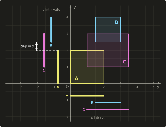
- A = [0, 2] × [0, 2] and B = [1.5, 3] × [2.5, 4]: in x, and , overlap; in y, fails. No collision, although the x intervals overlap.
- A and C = [1, 3.5] × [1, 3]: x overlaps (, ), y overlaps (, ). Overlap.
- B and C: x (, ) and y (, ) both overlap. Overlap.
Tunneling and continuous collision detection
Testing only at the end of each step misses fast, thin things.
A bullet-like ball of radius 0.1 m flying at 30 m/s moves m per 60 Hz step.
A wall 0.2 m thick plus the ball's diameter is only 0.4 m, so the ball can be in front of the wall in one step and behind it in the next, never overlapping: tunneling (すり抜け).
Fixes are smaller steps, thicker collision shapes, or continuous collision detection (CCD, 連続衝突検出), which tests the whole swept path of the step (for the ball, a capsule from the old to the new position) and finds the time of impact.
Response: restitution and impulses
Once a contact is found, collision response (衝突応答) changes the velocities so the bodies separate.
Because a collision takes almost no time, it's modeled as an impulse (力積) , an instant change of momentum, along the contact normal.
The coefficient of restitution (反発係数) says how much of the approaching speed comes back:
is a perfectly elastic bounce (no energy lost), a perfectly inelastic one (the bodies stick together), and real materials lie in between (a tennis ball around 0.7 to 0.8).
In 1D, for two bodies with velocities , and the relative velocity , the impulse that achieves this while conserving momentum is
Worked example.
kg moves right at m/s, kg moves left at m/s, and .
, so
Check: the new relative velocity is ; the momentum is before and after; the kinetic energy drops from J to J.
A ball bouncing on the (infinitely heavy) ground keeps the fraction of its speed, and since the height of a throw is proportional to the speed squared, each bounce reaches of the previous height: with , a drop from 1 m comes back to 0.64 m.
In 3D the same formula is applied along the contact normal (rotation adds terms with the inertia tensor), friction (摩擦) adds an impulse along the surface, and the bodies are pushed apart by the penetration depth.
Constraints
Many things aren't free: a door is attached to its hinge, a chain's links must stay connected, a character's bones are joined.
Constraints (拘束) restrict the motion: a ball joint keeps two points together, a hinge allows rotation about one axis only, a distance constraint keeps a length.
Physics engines solve all contacts and constraints together each step, usually iteratively, a few passes that each correct a little.
A ragdoll (ラグドール) is a character skeleton (chapter 13) turned into rigid bodies connected by joint constraints with angle limits, which is how game characters fall convincingly.
14.7 Fluids, smoke, fire and destruction
Two ways to describe a fluid
Water, smoke and fire are fluids (流体).
Their motion is described by the Navier–Stokes equations (ナビエ・ストークス方程式): for every small piece of fluid, with pressure, viscosity (粘性) and external forces, plus the condition that the fluid is incompressible (非圧縮性).
We won't derive them; what matters is that simulators discretize the fluid in one of two ways:
- Eulerian grids (格子法, オイラー的手法): fixed cells store velocity, pressure, density and temperature; the fluid flows through the grid. Natural for smoke and fire. Jos Stam's "Stable Fluids" (SIGGRAPH 1999) made grid fluids practical for graphics with a step that is stable for any time step. The cost is memory: cells are already 16.8 million.
- Lagrangian particles (粒子法, ラグランジュ的手法): particles carry mass and velocity and move with the flow. Natural for splashing water, and mass is automatically conserved. The best-known method is SPH (smoothed particle hydrodynamics, 平滑化粒子流体力学法), developed in 1977 for astrophysics by Gingold and Monaghan and, independently, by Lucy. Each quantity is a weighted sum over nearby particles; for example the density at particle is with a smooth kernel that falls to zero at a radius. Müller, Charypar and Gross (2003) brought SPH to interactive graphics.
Film water often combines both (hybrid PIC/FLIP methods).
For rendering, the liquid surface is rebuilt from the particles as an implicit surface and polygonized with marching cubes (chapter 9, section 9.3), and smoke is rendered as a participating medium with volume rendering (chapter 12, section 12.6).
Destruction
Breaking things is usually rigid-body simulation with a trick: before the simulation, the object is pre-fractured into pieces (often with a 3D Voronoi diagram scattered around the impact point), and the pieces are glued together with breakable constraints.
When an impulse exceeds a constraint's strength, the glue breaks and the pieces fly as independent rigid bodies, with particles for dust on top.
Exam points
- Explicit Euler uses only the old state; it is first order and adds energy to an undamped oscillator for every step size (factor per step), so it can blow up.
- Semi-implicit (symplectic) Euler updates the velocity first: same cost, bounded energy, stable for . Implicit Euler is stable for any step but damps. RK4 is fourth order and costs four evaluations. Stiff springs need small steps, substeps or implicit integration.
- Mass–spring cloth: structural, shear and bend springs; Hooke's law.
- Collision detection: broad phase, then narrow phase; two AABBs overlap only if they overlap on every axis; tunneling and CCD. Response: restitution coefficient (1 elastic, 0 inelastic), impulse along the normal, momentum conserved.
- Fluids: Eulerian grids vs Lagrangian particles (SPH).
14.8 Real-time animation
The frame budget
In real-time animation (リアルタイムアニメーション), every frame must be finished before the display wants the next one.
At a frame rate of frames per second, the frame budget (フレーム時間の予算) is ms:
| Frame rate | Budget per frame |
|---|---|
| 30 fps | 33.3 ms |
| 60 fps | 16.7 ms |
| 90 fps (VR headsets) | 11.1 ms |
| 120 fps | 8.33 ms |
| 144 fps | 6.94 ms |
Input, game logic, animation, physics, audio and rendering all share these 16.7 ms (the CPU and GPU work in parallel, so each has roughly its own budget).
Offline rendering may spend hours on a frame; a game must decide everything per frame, while the player presses buttons, so expensive effects are often baked: simulated offline and played back as animation.
| Offline (film) | Real-time (games, VR) | |
|---|---|---|
| Time per frame | minutes to hours | a few milliseconds |
| Input | fixed in advance | the user, every frame |
| Simulation | high resolution, can be rerun and art-directed | low resolution, must never explode, often baked |
| Characters | full rig, any deformation | skeleton + GPU skinning, LOD |
The game loop and the fixed time step
A game runs a game loop (ゲームループ): read input, update the world, render, repeat.
The simplest version advances the simulation by the measured frame time.
That makes the physics depend on the frame rate: a slow frame of 100 ms is a huge step (remember the exploding spring), and results differ between fast and slow computers.
The standard fix is a fixed time step (固定時間刻み): the simulation always advances by the same , as many times as needed to catch up with real time, using an accumulator:
- Add the frame's real elapsed time to the accumulator.
- While the accumulator holds at least : save the current state as the previous state, run one simulation step, subtract .
- Render a state interpolated between the previous and the current state with : .
Worked example.
Physics runs at 50 Hz ( ms) and the display at 60 fps (frames of ms).
| Frame | Accumulator after adding | Steps | Left over | |
|---|---|---|---|---|
| 1 | 16.67 | 0 | 16.67 | 0.83 |
| 2 | 33.33 | 1 | 13.33 | 0.67 |
| 3 | 30.00 | 1 | 10.00 | 0.50 |
| 4 | 26.67 | 1 | 6.67 | 0.33 |
| 5 | 23.33 | 1 | 3.33 | 0.17 |
| 6 | 20.00 | 1 | 0.00 | 0 |
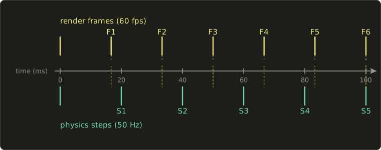
In 100 ms, 6 frames and exactly 5 steps of 20 ms: the simulation keeps pace with real time.
Without interpolation, frame 1 would show no motion and frames 2 to 6 one step each: a stutter.
With it, the motion is smooth, at the cost of showing the world up to one step late.
If a frame takes very long, the loop must cap the number of steps per frame; otherwise the steps take even longer, the next frame has to catch up even more, and the game freezes (the "spiral of death").
#include <cstdio>

// A ball falling under gravity, simulated with a FIXED time step and drawn at any frame rate.
struct State {
  double y, v;
};

State step(State s, double h) {           // semi-implicit Euler, g = 9.8 m/s^2
  double v = s.v - 9.8 * h;
  return {s.y + h * v, v};
}

int main() {
  const double h = 0.020;                 // physics: 50 steps per second
  const double frameTimes[] = {1 / 60.0, 1 / 60.0, 1 / 60.0, 1 / 60.0, 1 / 60.0, 0.100, 1 / 60.0};
  const int maxStepsPerFrame = 4;         // protection against the "spiral of death"

  State previous{10.0, 0.0}, current{10.0, 0.0};
  double accumulator = 0.0;
  int frame = 0;
  for (double frameTime : frameTimes) {   // in a game: measured with a clock
    accumulator += frameTime;
    int steps = 0;
    while (accumulator >= h && steps < maxStepsPerFrame) {
      previous = current;
      current = step(current, h);
      accumulator -= h;
      ++steps;
    }
    if (steps == maxStepsPerFrame && accumulator >= h) {
      accumulator = 0.0;                  // too far behind: drop the rest
    }
    double alpha = accumulator / h;       // how far we are between previous and current
    double yDraw = (1 - alpha) * previous.y + alpha * current.y;
    printf("frame %d: steps %d, alpha %.3f, draw y = %.4f\n", ++frame, steps, alpha, yDraw);
  }
  return 0;
}
frame 1: steps 0, alpha 0.833, draw y = 10.0000
frame 2: steps 1, alpha 0.667, draw y = 9.9974
frame 3: steps 1, alpha 0.500, draw y = 9.9922
frame 4: steps 1, alpha 0.333, draw y = 9.9843
frame 5: steps 1, alpha 0.167, draw y = 9.9739
frame 6: steps 4, alpha 0.000, draw y = 9.8902
frame 7: steps 0, alpha 0.833, draw y = 9.8641
Frames 1 to 5 match the table.
Frame 6 is a 100 ms hitch: 103.3 ms are waiting, which would be 5 steps, but the cap allows 4 and the rest is dropped, so the game runs a little slow for a moment instead of freezing.
You'll write a loop like this yourself in the OpenGL series, chapter 26.
Playing back skeletal animation
The keyframed or motion-captured clips of chapter 13 are played in a game by sampling each clip at the current time, every frame, for every joint.
A character rarely plays one clip alone:
- Animation blending (アニメーションブレンド, the motion blending of section 13.9): mix two clips per joint with a weight, interpolating rotations with slerp or normalized lerp. A walk at 1.5 m/s and a run at 4.5 m/s blended with the weight give a jog at 2.5 m/s. If one hip angle is 20° in the walk and 50° in the run, the blend gives . The two cycles must be time-aligned (same foot down at the same phase), or the feet slide.
- Cross-fades (クロスフェード): when switching clips, blend from the old to the new over 0.2 to 0.3 s instead of jumping.
- Animation state machines (アニメーションステートマシン): states such as idle, walk, run, jump, with transitions triggered by game events and conditions ("speed > 0.1", "jump pressed").
- Blend trees (ブレンドツリー): a tree of blend nodes driven by parameters, for example speed and direction blending eight locomotion clips at once.
- Layers and IK: additive layers (breathing, recoil), an upper body that aims while the legs run, and inverse kinematics (chapter 13) that puts the feet on uneven ground at runtime.
GPU skinning and animation LOD
Games run the skinning of chapter 13 (section 13.8) in the vertex shader, with the bone matrices uploaded once per frame: GPU skinning (GPUスキニング).
A character with 10,000 vertices and 4 influences per vertex needs 40,000 matrix–vector products per frame; 200 characters at 60 fps make per second, easy for a GPU, painful for a CPU.
Animation LOD (アニメーションのLOD) applies the level-of-detail idea of chapter 9 to motion: distant characters update their skeletons less often, use fewer bones, or switch to baked vertex animation.
200 characters with 60 bones at 60 Hz need joint updates per second.
If 150 of them are far away and update at 15 Hz, it's , less than half.
Physics engines and interaction
Games use physics engines (物理エンジン), libraries for rigid bodies, collisions, constraints, character controllers and vehicles, with a fixed time step and semi-implicit integration.
Their first rule is robustness: a game simulation must never explode, even when a player drives a truck into a hundred stacked crates.
Real-time animation is also interactive (インタラクティブ): the player's input changes the motion every frame, so characters combine responsive state machines with physics for secondary motion and ragdolls.
A simple 3D character controller with collisions is built in the OpenGL series, chapter 37; the hardware side of real-time systems (GPUs, V-sync, latency) is chapter 17.
14.9 Procedural animation
Procedural animation (手続き型アニメーション) computes motion from a rule or a function instead of keys or a physics simulation.
It needs very little data, it can be changed with a few parameters, and it never repeats exactly.
Motion from functions
- Oscillation: a buoy bobbing on the sea, . With m and Hz it's at 0.2 m at s, at 0 at s and at −0.2 m at s.
- Traveling waves: add a phase that depends on the position, , and a field of grass or a row of flags sways as a wave that moves with the speed : with rad/s and rad/m, 4 m/s.
- Noise-driven motion (ノイズによる動き): sample the noise of chapter 11, section 11.10 with time as the input instead of position. A camera shake that moves the camera by m, with the value noise of chapter 11, is at m at s (the worked example there had ). It wanders smoothly without repeating, which is exactly what a hand-held camera, a flickering flame or an idle creature should do. Several octaves give jitter on top of slow drift.
- Procedural walk cycles: the feet follow arcs from footstep to footstep, placed with IK (chapter 13), and the hips bob twice per cycle (once per step). Spiders and robots with many legs are often animated entirely this way.
Expressions and drivers
DCC tools (Maya, Blender, Houdini and others) let you attach a small formula, an expression (エクスプレッション) or driver (ドライバー), to any parameter.
The classic example: a wheel that rolls without slipping turns by radians when it travels the distance .
A car moving 3 m with wheels of radius 0.3 m turns them by rad , about 1.59 turns, automatically, whatever path the animator gives the car.
Flocking: boids
In 1987, Craig Reynolds published "Flocks, Herds, and Schools: A Distributed Behavioral Model" (SIGGRAPH '87).
Instead of scripting a flock's path, he simulated each bird, a boid (ボイド, from "bird-oid"), as an independent agent that sees only its nearby flockmates and follows three simple steering rules:
- Separation (分離; Reynolds called it collision avoidance): steer away from flockmates that are too close.
- Alignment (整列; velocity matching): steer toward the average velocity (heading and speed) of the neighbors.
- Cohesion (結合; flock centering): steer toward the average position (center) of the neighbors.
Reynolds gave them in this order of priority: avoiding collisions matters most.
No boid knows the shape of the whole flock and there is no leader; the flock's behavior, splitting around obstacles and merging again, emerges from the local rules.
That makes it a classic example of behavioral animation (行動のアニメーション, ビヘイビアアニメーション).
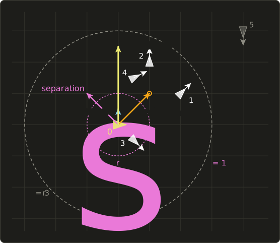
Worked example.
Boid 0 is at with velocity .
It sees neighbors within the radius , and treats neighbors closer than as too close.
The other boids:
| Boid | Position | Velocity | Distance to boid 0 |
|---|---|---|---|
| 1 | |||
| 2 | |||
| 3 | |||
| 4 | |||
| 5 | 5: not a neighbor |
- Cohesion: the center of boids 1 to 4 is . Steering: center minus own position, .
- Alignment: the average velocity is . Steering: average minus own velocity, .
- Separation: only boid 3 is closer than 1. Steering away from it, weighted by the inverse square distance: .
With all three weights equal to 1, the total steering is : straight up, away from boid 3 below and toward the group above.
Applied as an acceleration for one step s: , a turn of to the left, and .
Real implementations weight separation most and limit the speed and the turning rate.
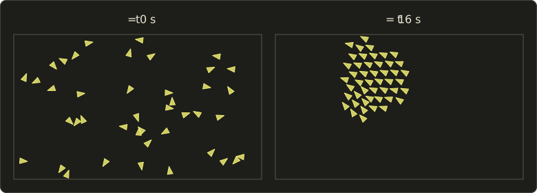
Run these rules for every boid, every step, and random scattered boids organize themselves into a flock.
This picture is a 2D simulation of 48 boids with the same radii (weights 1.5, 1 and 0.6, speed limited to between 1.5 and 3, semi-implicit Euler with s):
The cost is in finding the neighbors: naively every boid checks every other (), so real flocks use a grid or another spatial structure, as in the broad phase of section 14.6.
Crowds
Crowd simulation (群衆シミュレーション) extends the idea to people: each agent (エージェント) has a goal, plans a path, avoids other agents locally, and an animation system picks clips to match its motion.
Crowd tools like Massive, developed for the battle scenes of the Lord of the Rings films, gave each agent simple perception and decision rules, so thousands of soldiers could fight without an animator touching each one; games use heavy LOD, down to animated billboards for distant crowds.
Growing plants: L-systems over time
The generations of the L-systems of chapter 9, section 9.5 jump when shown one after the other.
To animate growth, each module gets an age, and its length, width and angle are smooth functions of the age, so the plant grows continuously, new branches sprouting while older ones thicken.
Exam points
- Frame budget = 1000 / fps ms (16.7 ms at 60 fps). A fixed time step with an accumulator keeps physics independent of the frame rate; render by interpolating between the last two states.
- Real-time characters: blending (with slerp), cross-fades, state machines, blend trees, GPU skinning in the vertex shader, animation LOD.
- Procedural animation: motion from rules or functions (sine waves, noise over time, expressions such as ).
- Boids (Reynolds 1987): separation, alignment, cohesion, using only nearby flockmates; no leader. Alignment matches the velocity, cohesion moves toward the center.
14.10 Compositing with live action
The VFX flow
A visual-effects (VFX) shot puts CG into footage shot with a real camera: a creature in a real street, a set extension behind real actors.
The footage is the plate (プレート, 実写素材), and combining the layers into one image is compositing (合成, コンポジット).
For the result to be believable, the CG must match the plate in every way the camera model of chapter 2 describes: the camera's position and lens, the light, the motion blur, the focus and the noise.
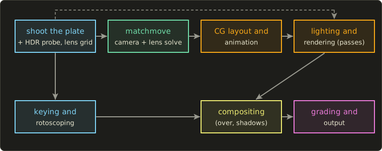
On set, the crew records the lens data, photographs a lens grid to measure the distortion, and shoots an HDR light probe where the CG object will stand.
Matchmoving: recovering the camera
Matchmoving (マッチムーブ), also called camera tracking (カメラトラッキング), recovers the real camera's motion from the footage, so the CG camera can copy it exactly.
It works in two parts:
- 2D tracking: follow many distinct points (corners, markers placed on set) from frame to frame through the image.
- Camera solve: find, for every frame, the camera's position and orientation, and the focal length (and lens distortion), together with the 3D positions of the tracked points, so that projecting the 3D points through the pinhole model of chapter 2, section 2.2 lands on the tracked 2D positions. This is the structure from motion problem of computer vision.
The solver measures its quality with the reprojection error (再投影誤差).
Say the camera has a 35 mm lens on a 36 mm wide sensor and the image is 1920 pixels wide, so the focal length in pixels is px.
A solved 3D point at in camera space (the camera looks down −z) projects to
from the image center.
If the tracker measured the feature at , the error is , about px.
The solver adjusts all cameras and points to minimize the sum of the squared errors over all points and frames; a good solve has an average error well below one pixel, and CG locked to it doesn't "slide" on the plate.
Matchmoving recovers the camera (and a sparse cloud of points); it doesn't separate the actors from the background, which is the next job.
The plate also has the real lens's distortion (歪曲収差), while the renderer's pinhole camera has none.
So the plate is undistorted with the measured model (chapter 2: ) for tracking, the CG is rendered undistorted, and the finished CG is redistorted with the same model before it's combined with the original plate.
With , a CG point rendered at the normalized radius must move to to sit where the real lens would have put it.
When the move is planned in advance, a motion control camera (モーションコントロールカメラ) on a robotic rig can repeat exactly the same move many times (actors, clean background, miniatures); the Dykstraflex built for Star Wars (1977) is the famous early example.
Chroma key
To put an actor into a CG world, we need a matte (マット): an alpha channel saying which pixels belong to the actor (chapter 2 introduced alpha as the fourth channel).
The classic way is to shoot the actor in front of a uniform, strongly colored screen and compute the matte from the color: chroma key (クロマキー), and the process of pulling a matte is keying (キーイング).
The screen is green (グリーンバック) or blue (ブルーバック), the colors farthest from skin tones; green gives the cleanest channel on a Bayer sensor (chapter 2, section 2.4, twice as many green photosites), blue is used when the costume is green.
A simple and widely used keyer is the color difference method: how much greener is a pixel than its other channels?
where is the same difference for the screen color.
For a screen color , .
- The screen itself: , (fully transparent).
- Skin : , clamped to 0, (opaque).
- An edge pixel half covered by a gray sweater : the camera averages , so and : exactly right.
- Half skin, half screen: , , instead of the true 0.5. The method is exact only for neutral colors; real keyers have many controls to tune such cases.
The edge pixel still contains half of the green screen.
Screen subtraction removes it: subtracting leaves the foreground's contribution,
which is the sweater color multiplied by its alpha: a premultiplied color (below).
Composited over a new blue-sky background : .
Green light bouncing off the screen also tints the actor's edges and shiny surfaces: spill (スピル).
Spill suppression (スピル除去) limits the green channel where it's higher than the other channels justify, for example
Skin has and stays unchanged; skin with spill, , becomes .
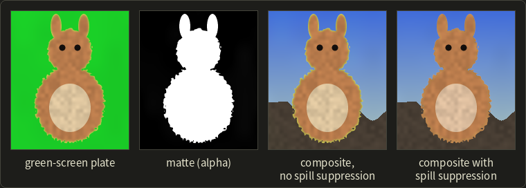
The creature, the screen and the background in this picture are all generated (no photos).
The plate mixes the creature's true coverage with the slightly uneven screen, and adds green spill near the outline.
The keyer above recovers the matte with an average error of less than 0.01 per pixel; the third panel shows the green fringe that spill leaves, and the fourth the result with spill suppression.
The same steps as a fragment shader function (Slang first, then GLSL, then HLSL):
static const float3 screenColor = float3(0.1, 0.8, 0.15);

float keyAlpha(float3 c) {
  float d = c.g - max(c.r, c.b);
  float dS = screenColor.g - max(screenColor.r, screenColor.b);
  return 1.0 - saturate(d / dS);
}

// The keyed foreground: premultiplied color in rgb, alpha in a.
float4 keyPixel(float3 plate) {
  float a = keyAlpha(plate);
  float3 fg = max(plate - (1.0 - a) * screenColor, float3(0.0, 0.0, 0.0)); // screen subtraction
  fg.g = min(fg.g, 0.5 * (fg.r + fg.b));                                    // spill suppression
  return float4(fg, a);
}

// Premultiplied "over": foreground over an opaque background.
float3 over(float4 fg, float3 background) {
  return fg.rgb + (1.0 - fg.a) * background;
}
const vec3 screenColor = vec3(0.1, 0.8, 0.15);
float keyAlpha(vec3 c) {
float d = c.g - max(c.r, c.b);
float dS = screenColor.g - max(screenColor.r, screenColor.b);
return 1.0 - clamp(d / dS, 0.0, 1.0);
}
// The keyed foreground: premultiplied color in rgb, alpha in a.
vec4 keyPixel(vec3 plate) {
float a = keyAlpha(plate);
vec3 fg = max(plate - (1.0 - a) * screenColor, vec3(0.0)); // screen subtraction
fg.g = min(fg.g, 0.5 * (fg.r + fg.b)); // spill suppression
return vec4(fg, a);
}
// Premultiplied "over": foreground over an opaque background.
vec3 over(vec4 fg, vec3 background) {
return fg.rgb + (1.0 - fg.a) * background;
}static const float3 screenColor = float3(0.1, 0.8, 0.15);
float keyAlpha(float3 c) {
float d = c.g - max(c.r, c.b);
float dS = screenColor.g - max(screenColor.r, screenColor.b);
return 1.0 - saturate(d / dS);
}
// The keyed foreground: premultiplied color in rgb, alpha in a.
float4 keyPixel(float3 plate) {
float a = keyAlpha(plate);
float3 fg = max(plate - (1.0 - a) * screenColor, float3(0.0, 0.0, 0.0)); // screen subtraction
fg.g = min(fg.g, 0.5 * (fg.r + fg.b)); // spill suppression
return float4(fg, a);
}
// Premultiplied "over": foreground over an opaque background.
float3 over(float4 fg, float3 background) {
return fg.rgb + (1.0 - fg.a) * background;
}
Spill suppression on the premultiplied color is fine: scaling all three channels by doesn't change which one is larger.
Keying is part of image editing in general; the filters that clean up a matte (blur, erode, dilate) are in chapter 15.
Mattes, alpha and premultiplication
Chapter 10, section 10.12 blended a surface over the frame buffer with the over operator, .
Compositing needs the full version, in which the background may itself be partly transparent (a layer, not the final image).
Porter and Duff (1984) defined it with premultiplied alpha (乗算済みアルファ, プリマルチプライドアルファ): store each pixel as instead of .
Writing for the premultiplied color, A over B is
The same formula for all four channels.
Premultiplied alpha is the standard inside compositors and renderers, for three reasons:
- Filtering is correct. Average a red opaque pixel with a transparent neighbor whose invisible color happens to be green, , as scaling or blurring does. Straight: , which over white gives , a yellowish fringe. Premultiplied, the transparent pixel is , the average , and over white : pink, half red over white, as it should be.
- "Over" is associative: , so layers can be precombined in any grouping.
- Additive light works: a pixel with but a nonzero color adds light without covering anything (a glow).
Porter and Duff also defined in, out, atop and xor for combining mattes.
A garbage matte (ガベージマット) is drawn roughly by hand to throw away unwanted areas (a light stand at the edge of the screen); a holdout matte (ホールドアウトマット) cuts the CG where a real object passes in front of it.
Rotoscoping
Not every shot has a green screen.
Rotoscoping (ロトスコープ) creates the matte by hand: an artist draws spline shapes around the object in key frames, the software interpolates and tracks them, and the artist corrects them frame by frame.
The name comes from Max Fleischer's rotoscope (patented in 1917), a device for tracing live-action film frame by frame for cartoons.
Rotoscoping is slow but works on any footage; chroma key is automatic but needs a colored screen when shooting.
| Chroma key | Rotoscoping | Matchmoving | |
|---|---|---|---|
| Produces | a matte (alpha) | a matte (alpha) | the camera (position, orientation, focal length) and 3D points |
| From | the color of each pixel | shapes drawn by an artist, frame by frame | 2D features tracked through the frames |
| Needs at shooting time | a blue or green screen | nothing special | trackable features, lens data |
Matching the light, the shadows and the camera
Even with a perfect camera and matte, CG looks pasted on unless its light matches the plate:
- Light: the HDR light probe shot on set lights the CG with image-based lighting, as in chapter 12, section 12.13, so it receives the same light from the same directions. The white balance and color temperature must match the plate's (chapter 3, section 3.8).
- Shadows and contact: a CG creature must cast shadows on the real ground. A simple stand-in model of the ground is rendered as a shadow catcher (シャドウキャッチャー): invisible itself, it only records the shadow (and reflections) that the CG casts on it. Debevec's differential rendering (差分レンダリング, 1998) adds to the plate the difference the object makes: render the local scene with and without the object and add (with − without). A plate pixel of 0.6 where the local model renders 0.5 without the creature and 0.3 with its shadow becomes , darkened by exactly the shadow, while the plate's own texture stays.
- Render passes (レンダーパス, AOV): separate images (diffuse, specular, shadow, depth, motion vectors) let the compositor adjust each part without re-rendering.
- Camera effects: CG is perfectly sharp and clean; the plate is not. The compositor matches motion blur (the real shutter time, chapter 2, section 2.3), depth of field and lens effects, and adds the plate's grain (粒状感, フィルムグレイン). A final color grade (グレーディング) unifies the shot.
Virtual production
Virtual production (バーチャルプロダクション) moves part of compositing onto the set.
The actors stand in an LED volume, a stage surrounded by large LED walls, on which a real-time engine renders the CG environment from the tracked camera's point of view, with correct parallax, while the camera films the actors and the screen together: "in-camera VFX".
ILM's StageCraft for The Mandalorian (2019, rendered with Unreal Engine) made the technique famous.
The LED walls also light the actors with the environment's colors and give real reflections on shiny costumes, with no green spill to remove; on the other hand the walls' resolution and brightness are limited, and moiré appears if the camera focuses on the LED pixels (sampling again, chapter 2).
Exam points
- Matchmoving (camera tracking) recovers the real camera's position, orientation and focal length (and lens distortion) for every frame, from 2D features tracked in the footage; quality = reprojection error. CG is rendered undistorted, then redistorted.
- Chroma key computes a matte from the color of a blue or green screen; spill is screen light on the subject and is suppressed by limiting the green channel. Rotoscoping draws the matte by hand, frame by frame, and needs no screen.
- Premultiplied alpha stores ; over: . It filters correctly and is associative.
- Lighting match uses an HDR light probe (IBL); shadow catchers and differential rendering add CG shadows to the plate; motion blur, depth of field and grain must match the plate.
14.11 Summary
- Physics-based animation advances a state (position, velocity) with and a numerical integrator: plausible motion automatically, but hard to direct.
- Explicit Euler adds energy to oscillators for any step size; semi-implicit Euler costs the same and stays bounded while ; Verlet is second order, RK4 fourth order; implicit Euler is always stable but damps.
- Particle systems emit, move, collide, age and kill particles; mass–spring systems model cloth, soft bodies and hair; rigid bodies add orientation, torque and the inertia tensor; collisions need a broad and a narrow phase and are resolved with impulses; fluids use grids or particles (SPH).
- Real-time animation fits into the frame budget (16.7 ms at 60 fps) with a fixed time step and interpolation, blended clips, GPU skinning and animation LOD.
- Procedural animation computes motion from rules: sine waves, noise over time, expressions, boids (separation, alignment, cohesion), crowds, growing L-systems.
- Compositing matches CG to the plate: matchmoving and lens distortion for the camera, chroma key or rotoscoping for mattes, premultiplied "over", HDR probes and shadow catchers for light and shadow, motion blur and grain for the look.
14.12 Key terms
| English | 日本語 |
|---|---|
| physics-based animation | 物理ベースアニメーション |
| simulation | シミュレーション |
| state | 状態 |
| equation of motion | 運動方程式 |
| time step | 時間刻み |
| numerical integration | 数値積分 |
| explicit Euler method | 陽的オイラー法(前進オイラー法) |
| semi-implicit (symplectic) Euler method | 半陰的オイラー法(シンプレクティックオイラー法) |
| Verlet method | ベルレ法 |
| Runge–Kutta method | ルンゲ=クッタ法 |
| implicit Euler method | 陰的オイラー法 |
| stability | 安定性 |
| damping | 減衰(ダンピング) |
| critical damping | 臨界減衰 |
| particle system | パーティクルシステム |
| emitter | エミッタ |
| mass–spring system | バネ質点系 |
| Hooke's law | フックの法則 |
| rest length | 自然長 |
| structural, shear and bend springs | 構造バネ、せん断バネ、曲げバネ |
| deformable body, soft body | 変形体、ソフトボディ(弾性体) |
| rigid body | 剛体 |
| center of mass | 重心 |
| angular velocity | 角速度 |
| torque | トルク |
| inertia tensor | 慣性テンソル |
| collision detection | 衝突検出(衝突判定) |
| broad phase, narrow phase | ブロードフェーズ、ナローフェーズ |
| bounding sphere | 境界球(バウンディングスフィア) |
| axis-aligned bounding box (AABB) | 軸平行境界ボックス(AABB) |
| tunneling | すり抜け |
| continuous collision detection | 連続衝突検出 |
| collision response | 衝突応答 |
| impulse | 力積 |
| coefficient of restitution | 反発係数 |
| constraint | 拘束 |
| ragdoll | ラグドール |
| fluid | 流体 |
| Navier–Stokes equations | ナビエ・ストークス方程式 |
| Eulerian grid, Lagrangian particles | 格子法(オイラー的手法)、粒子法(ラグランジュ的手法) |
| smoothed particle hydrodynamics (SPH) | SPH(平滑化粒子流体力学法) |
| real-time animation | リアルタイムアニメーション |
| frame budget | フレーム時間の予算 |
| game loop | ゲームループ |
| fixed time step | 固定時間刻み |
| animation blending | アニメーションブレンド |
| animation state machine | アニメーションステートマシン |
| blend tree | ブレンドツリー |
| GPU skinning | GPUスキニング |
| physics engine | 物理エンジン |
| procedural animation | 手続き型アニメーション |
| expression, driver | エクスプレッション、ドライバー |
| flocking, boids | 群れ、ボイド |
| separation, alignment, cohesion | 分離、整列、結合 |
| behavioral animation | 行動のアニメーション(ビヘイビアアニメーション) |
| crowd simulation | 群衆シミュレーション |
| compositing with live action | 実写映像との合成 |
| plate | プレート(実写素材) |
| matchmoving, camera tracking | マッチムーブ、カメラトラッキング |
| reprojection error | 再投影誤差 |
| motion control camera | モーションコントロールカメラ |
| chroma key, keying | クロマキー、キーイング |
| blue screen, green screen | ブルーバック、グリーンバック |
| spill, spill suppression | スピル、スピル除去 |
| matte | マット |
| premultiplied alpha | 乗算済みアルファ(プリマルチプライドアルファ) |
| garbage matte, holdout matte | ガベージマット、ホールドアウトマット |
| rotoscoping | ロトスコープ |
| shadow catcher | シャドウキャッチャー |
| differential rendering | 差分レンダリング |
| render pass (AOV) | レンダーパス(AOV) |
| grain | 粒状感(フィルムグレイン) |
| virtual production | バーチャルプロダクション |
14.13 Challenges
- ★ A ball is thrown straight up from with m/s ( m/s², s). Compute three steps with explicit Euler and with semi-implicit Euler, and compare both with the exact height at s. Which one is too high, and why?
- ★ Give the frame budget in ms at 30, 90 and 144 fps. A game runs its physics at 120 Hz on a display that shows 50 fps: following the accumulator method of section 14.8, how many physics steps run in each of the first three frames, and what is after each?
- ★★ Two bodies collide head-on in 1D: kg at m/s and kg at rest. Compute the impulse and both final velocities for and for , and check the momentum and the kinetic energy in each case.
- ★★ A 1 kg mass hangs on a spring with N/m. What is the largest stable step for semi-implicit Euler? By what factor does explicit Euler multiply the energy per step at s, and after one second? How many substeps per 60 Hz frame does semi-implicit Euler need for N/m?
- ★★ A boid at flies with (, , all weights 1). The others: with velocity ; with ; with ; with ; with . Compute the cohesion, alignment and separation vectors and their sum, and explain in words what the boid will do.
- ★★★ Show with the premultiplied formula that "over" is associative, , for the colors and for alpha. Then explain why a costume with green parts is a problem for chroma key, and list three ways a production could handle it.
Multiple choice
Q1 ★ Which of the following statements about numerical integration in physics-based animation is correct?
| A | Explicit Euler keeps the energy of an undamped spring exactly constant, whatever the time step. |
| B | Making the time step larger always makes a simulation more accurate, because fewer steps accumulate less error. |
| C | With explicit Euler, the energy of an undamped spring grows every step, so the motion can blow up; a smaller time step or semi-implicit Euler helps. |
| D | Semi-implicit Euler is stable for any time step, however stiff the spring. |
| E | The fourth-order Runge–Kutta method needs only one force evaluation per step, like Euler. |
Q2 ★ Which of the following statements about Reynolds' boids is correct?
| A | Each boid steers using only its nearby flockmates, following separation, alignment and cohesion, and the behavior of the whole flock emerges from these local rules. |
| B | A leader boid computes the path of the whole flock and sends it to the other boids. |
| C | Alignment means steering toward the average position of the neighbors. |
| D | The boids model was first published by Reeves in 1983 as a particle system for fire. |
| E | Boids is a keyframe technique in which the animator sets every bird's position at every key. |
Q3 ★★ Which of the following pairs of a compositing technique and what it does is correct?
| A | Chroma key: estimates the real camera's motion from points tracked in the footage. |
| B | Rotoscoping: computes a matte automatically from the color of a blue or green screen. |
| C | Spill suppression: removes the lens distortion of the plate so that CG can be rendered with a pinhole camera. |
| D | Matchmoving: recovers the real camera's position, orientation and focal length for every frame, from features tracked in the footage, so the CG camera can copy it. |
| E | HDR light probe: records the shape of the set as a dense polygon mesh. |
14.14 Practical assignment
Simulate, bounce and composite a ball by hand.
You need paper (graph paper helps), a pencil and a calculator.
You'll run a tiny physics simulation, detect and resolve a collision, interpolate a frame, and key and composite a strip of pixels: the whole chapter on one sheet.
To keep the numbers easy, use m/s².
- Explicit vs semi-implicit. A ball (a point) is dropped from m with , time step s. Make a table with the columns step, , and , and compute the first three steps with explicit Euler and with semi-implicit Euler. Compare both with the exact .
- Fall and detect. Continue with semi-implicit Euler only. After each step, test for a collision with the ground: . Note the step at which it first happens and the penetration depth.
- Respond. At that step, set and replace the velocity with , using the restitution coefficient . Continue the table until the ball comes down a second time, and resolve that collision the same way.
- Compare with the theory. Find the highest in your table after the first bounce. Compute the exact impact speed for a drop from 2 m, the height an ideal bounce would reach ( m), and the height that the post-bounce speed of your table would reach exactly (). Explain the differences.
- Interpolate a frame. The display shows a frame at s, between steps 2 and 3. Compute and the drawn height by interpolating the semi-implicit states.
- Key a strip. A green-screen plate row has four pixels: , , and ; the screen color is . For each, compute , , and the premultiplied foreground .
- Composite. Composite each keyed pixel over the new background with the premultiplied "over". Then put a CG ball pixel, premultiplied with , over the third pixel twice: first as (ball over keyed pixel) over background, then as ball over (keyed pixel over background).
How to check yourself:
- Step 1: the exact height lies between the two methods; explicit Euler is too high and semi-implicit Euler too low by the same amount.
- Steps 2 and 3: the first collision is found at s with a small penetration (less than 0.2 m); every peak after a bounce is lower than the one before, and the total energy (per kg) never increases at a bounce.
- Step 4: your first peak after the bounce is below 1.28 m, and below for your post-bounce speed; the time step causes both the late detection and the lower peak.
- Step 5: , and the drawn height lies between the heights of steps 2 and 3.
- Step 6: the alphas are 0, 0.25, 0.75 and 1; every premultiplied foreground is gray, equal to , and no channel is larger than .
- Step 7: the opaque pixels show the background or the gray unchanged, and the two groupings of step 7 give the same color (associativity), with a resulting alpha of 1.
コメント(0)
まだコメントはありません。
ログインするとコメント出来ます。