16. Computational Photography, NPR and Visualization
So far, most of this series has aimed at one goal: a picture that looks like a photograph of a scene that doesn't exist.
This chapter is about three other ways of using the same machinery.
Computational photography turns the camera itself into a computer and makes photos that no single exposure could capture.
Non-photorealistic rendering deliberately draws pictures that don't look like photos: cartoons, technical illustrations, pen-and-ink drawings.
Visualization turns numbers (a CT scan, a flow simulation, a table of sales figures) into pictures that people can understand.
All three are about what a person should see rather than about physical accuracy, which is why the syllabus groups them as area 7, graphics that appeal to the eye (視覚に訴えるグラフィックス), with three items: computational photography (コンピュテーショナルフォトグラフィ), non-photorealistic rendering (ノンフォトリアリスティックレンダリング) and visualization (可視化).
Each part of the chapter ends with its own exam points.
Almost everything here reuses earlier chapters, so I'll link back instead of repeating: the camera, exposure and noise of chapter 2, color and perception from chapter 3, isosurfaces and marching cubes from chapter 9, shading and back faces from chapter 10, light fields from chapter 12, and tone mapping, convolution, edge detection and homographies from chapter 15.
16.1 What computational photography is
A classic camera is an optical instrument: the lens forms an image, the sensor records it once, and the photo is done.
Computational photography (コンピュテーショナルフォトグラフィ) treats capture and computation as one system.
It records more than one ordinary picture (several exposures, several focus settings, a light field, a coded blur) and then computes the photo it actually wants.
The result can have more dynamic range, more depth of field, less noise or less blur than any single exposure, or allow decisions (focus, lighting) to be changed after the shot.
It uses all three fields of section 2.11 (computer vision, image processing and the camera model), and its techniques can be sorted by what they change:
| What is changed | Techniques |
|---|---|
| exposure | HDR imaging, burst denoising, night modes |
| viewpoint | panoramas and image stitching |
| focus and optics | focus stacking, light field cameras, coded aperture |
| shutter | coded exposure, deblurring |
| lighting | flash/no-flash, image-based relighting |
| the image after capture | super-resolution, seam carving, synthetic depth of field |
Your phone does several of these every time you press the shutter button, usually without telling you.
16.2 HDR imaging from bracketed exposures
The problem: too much range for one exposure
Stand inside a room on a sunny day and photograph the window.
Either the room is exposed correctly and the window is a white blank, or the sky is exposed correctly and the room is black.
The dynamic range of the scene (the ratio of the brightest to the darkest part we care about) is larger than what one exposure can record.
A sunlit scene with deep shadows can exceed 100,000:1, about 17 stops (), and an 8-bit image file stores 256 levels.
The fix is to take several photos with different exposure times, a series called exposure bracketing (露出ブラケット), and merge them into one HDR image (high dynamic range, ハイダイナミックレンジ画像, chapter 2) that stores the scene's radiance as floating-point numbers.
The shutter speed is varied, not the aperture, because the aperture would also change the depth of field and make the photos disagree.
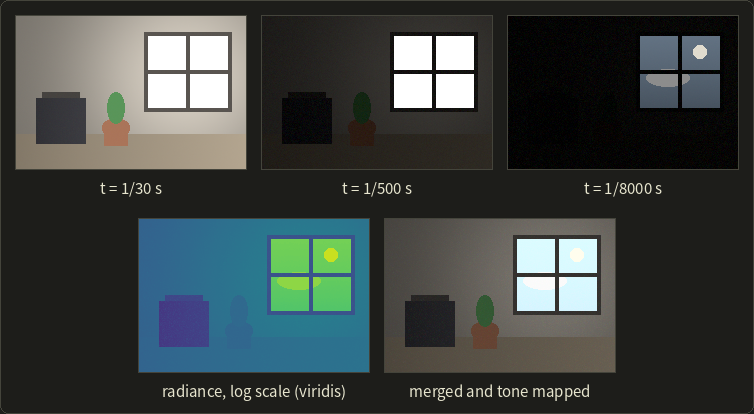
The synthetic scene spans 6,807:1 (12.7 stops) from the dark box to the sun, more than any single exposure holds.
The model
A camera turns the exposure (radiance times exposure time ) into a pixel value through its response curve (応答曲線) :
If we know , each exposure gives an estimate of the radiance at a pixel:
For RAW sensor data, is nearly linear and is simply (up to a constant).
A JPEG has been through a nonlinear curve (sRGB encoding at least, often more), and the camera doesn't tell you which.
Paul Debevec and Jitendra Malik ("Recovering High Dynamic Range Radiance Maps from Photographs", SIGGRAPH 1997) showed how to recover the curve from the bracketed photos themselves: the same scene point appears in every photo with a known ratio of exposure times, which gives enough equations to solve for (up to a scale).
They then merge the estimates with a weighted average of their logarithms:
The weight is a "hat", small near 0 (noise, quantization) and near 255 (clipping): for and above.
A saturated pixel () gets weight 0: it only tells us that the radiance was at least something.
Worked example: two exposures, two pixels
A camera with a linear response takes two shots, s and s, a ratio of 16, which is 4 stops.
Pixel P is in a shadow, pixel Q on a bright window:
| Pixel | (1/15 s) | (1/240 s) | ||||
|---|---|---|---|---|---|---|
| P | 80 | 6 | 1200 | 1440 | 80 | 6 |
| Q | 255 | 150 | (at least 3825) | 36,000 | 0 | 105 |
For P, the two estimates disagree: in the short exposure P is only 6 levels above black, so a noise of half a level is an 8% error.
The weights take care of it:
The result stays close to the reliable long exposure (averaging the values instead of their logarithms gives 1217, almost the same).
For Q the long exposure is clipped, so its weight is 0 and comes from the short exposure alone.
The merged image knows that Q is times brighter than P, while each single photo got one of them wrong.
In practice
Merging needs a static scene and camera: anything that moves between the shots appears several times (ghosting), so real software aligns the images first and rejects pixels that disagree.
The result is stored in a floating-point format such as OpenEXR and must be tone mapped (トーンマッピング, section 15.4) before an ordinary screen can show it.
The figure above uses one global curve (Reinhard's); local tone mapping (局所的なトーンマッピング) instead compresses only the large-scale brightness, for example an edge-preserving bilateral-filtered copy of the log luminance (chapter 15), and keeps the local detail, which gives many phone photos their "HDR look".
The light probes of section 12.13 are made exactly this way.
A renderer computes in floating point from the start, so games simply tone map every frame, as you'll do in the OpenGL series, chapter 21.
16.3 Panoramas: stitching several photos
A panorama (section 12.13 showed how it is viewed) is usually made by image stitching (画像のスティッチング): taking overlapping photos while turning the camera and combining them into one wide image.
The steps:
- Find feature points (特徴点) in every photo: distinctive spots such as corners, each with a descriptor of its neighborhood that survives rotation, scale and brightness changes (SIFT, David Lowe, 2004, is the classic).
- Match the features between overlapping photos by comparing descriptors.
- Estimate the transformation between each pair. When the camera only rotates about its optical center, or the scene is flat, two photos are related exactly by a homography (ホモグラフィ), the 3×3 projective transform of chapter 15. It has 9 entries but is defined only up to scale, so 8 unknowns; each matched point gives 2 equations, so 4 matches determine it.
- Reject wrong matches with RANSAC (Fischler and Bolles, 1981): pick 4 random matches, compute a homography, count how many other matches agree with it, repeat, and keep the best.
- Warp all photos onto a common surface (a plane for a few photos, a cylinder or sphere for a full turn).
- Blend the overlaps so that no seams show.
The number of RANSAC tries is easy to estimate.
If half of the matches are wrong, a random set of 4 is all correct with probability .
To find at least one clean set with 99% certainty we need tries with , that is : 72 tries, each of which costs almost nothing.
Blending.
The simplest blend is feathering: across the overlap, the weight of one photo falls linearly from 1 to 0 while the other's rises.
In a 100-pixel overlap, a pixel 25 pixels into it gets weights 0.75 and 0.25; if the photos show 120 and 140 there, the result is .
Multi-band blending (Burt and Adelson, 1983) blends the low frequencies over a wide zone and the fine details over a narrow one, using image pyramids; most stitching programs use it.
If the camera moves instead of only turning, near and far objects shift by different amounts (parallax), no single homography fits, and ghosts or broken lines appear.
16.4 Focus stacking, light field cameras and refocusing
Focus stacking
Section 2.3 showed that close-up photos have a very shallow depth of field.
Focus stacking (深度合成, フォーカススタッキング) takes several photos focused at different distances and keeps, for every pixel, the photo in which it's sharpest, measured for example by the local magnitude of the Laplacian (chapter 15): a focused region has strong high frequencies, a blurred one doesn't.
Light field cameras
Section 12.13 introduced the 4D light field, the radiance of every ray.
A light field camera (ライトフィールドカメラ, also plenoptic camera) captures a small one in a single shot by putting an array of tiny microlenses in front of the sensor (Ren Ng and colleagues at Stanford built a hand-held one in 2005).
Each microlens covers a small block of pixels, each of which sees the scene through a different part of the main lens's aperture, so the camera records both where a ray hits and which direction it came from.
The price is resolution.
Example: a 7680 × 5120 sensor (39.3 megapixels) with microlenses covering 10 × 10 pixels each gives 100 directions per position, but only positions: a 0.39-megapixel image.
That trade-off is why light field cameras stayed a niche, while phones achieve similar effects with depth estimation (section 16.6).
Refocusing by shift-and-add
Picking the same pixel from every microlens block gives one sub-aperture image: the scene seen through one small part of the lens, which is like a photo from a slightly shifted viewpoint.
A point in the plane of focus appears at the same position in every sub-aperture image; a point at another depth shifts from one sub-aperture image to the next, in proportion to the offset of the sub-aperture and its distance from the plane of focus.
Ordinary photography adds all sub-aperture images as they are, so off-focus points are smeared: that's defocus blur, computed.
Refocusing (リフォーカス) shifts each sub-aperture image before adding.
Example in 1D with three sub-apertures : point A is at , that is at pixels 8, 10 and 12.
Added as they are, A is spread over 8 to 12: blurred.
Shifting each image by moves all three copies to , and A is sharp, while a point that used to be sharp (same position in all three) is now spread over 4 pixels.
Choosing the shift per unit chooses the plane of focus after the photo was taken; averaging fewer sub-apertures gives a deeper depth of field, like stopping down.
16.5 Deblurring, coded aperture and coded exposure
Blur is a convolution
A camera that shakes during the exposure, or a subject that moves, smears every point into the same small shape, the point spread function (点像分布関数, PSF).
If the blur is the same everywhere, the blurred image is the sharp image convolved (畳み込み, chapter 15) with the PSF , plus noise :
Deblurring means undoing this: deconvolution (逆畳み込み, デコンボリューション).
When the PSF is known it's "non-blind" deconvolution; when it must be estimated from the blurry photo too, "blind" deconvolution, which is much harder.
Worked example: why deconvolution is fragile
Take a 1D signal (a sharp step) and motion blur over 3 pixels, , with zeros before the start:
The step became a ramp.
Inverting is just algebra: , which gives back exactly.
Now add a tiny bit of noise, 0.3 to the fourth sample only, so .
The same formula gives
and the error pattern repeats forever: a noise of 0.3 became an error of 0.9 that never dies out.
The reason is visible in the pattern itself: any sequence that repeats sums to zero over every 3 neighboring samples, so the blur erases it completely.
In the language of chapter 15, the box kernel's frequency response is zero at a frequency of 1/3 cycle per pixel, and dividing by (nearly) zero amplifies the noise at that frequency without limit.
Practical methods, such as the Wiener filter or Richardson–Lucy iteration, therefore don't divide blindly: they give up on frequencies where the signal is weaker than the noise.
Coded exposure and coded aperture
If the trouble is that the PSF has zeros in its frequency response, change the PSF.
Coded exposure (符号化露光; Raskar, Agrawal and Tumblin, "flutter shutter", 2006) opens and closes the shutter in a pseudo-random binary pattern during the exposure.
A moving object is then smeared into a dashed line instead of a box, and a well-chosen pattern has no zeros in its frequency response, so the motion blur becomes invertible.
Coded aperture (符号化開口; for example Levin, Fergus, Durand and Freeman, 2007) does the same for defocus: a patterned mask in the lens aperture makes the defocus PSF easier to invert, and because the pattern's size depends on depth, it also lets the computer estimate how far away each part of the scene is.
16.6 Flash, bursts and the smartphone camera
Burst photography: averaging away the noise
A pixel value is the true value plus random noise: the light itself arrives as a random number of photons, and the sensor's electronics add their own noise (section 2.3 showed that raising the sensitivity amplifies it).
Take photos of a static scene and average them.
The true value stays the same, while independent noise with standard deviation shrinks to
Example: a single frame has noise levels.
Averaging 4 frames gives , 9 frames , 16 frames .
To halve the noise you need four times as many frames; in decibels, 16 frames improve the signal-to-noise ratio by dB.
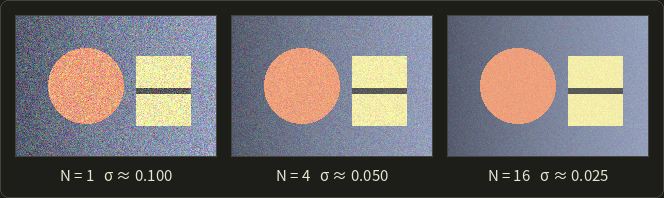
The measured noise in the picture (0.100, 0.050, 0.025) follows the formula exactly.
Why not just one long exposure with the same total light?
Because a hand-held long exposure is blurred (section 16.5) and bright parts clip; many short exposures avoid both, and the computer aligns them before averaging.
This is burst photography (バースト撮影), the core of smartphone "night modes": many frames over a second or more, aligned locally, merged robustly (a pixel that disagrees because something moved gets a low weight) and tone mapped.
Flash and no-flash
In a dim room, a flash photo is clean but flat and cold, a photo without flash has the room's mood but is noisy.
Flash/no-flash photography (Petschnigg et al., and Eisemann and Durand, both 2004) takes both: the colors and large-scale lighting come from the no-flash photo, the details and low noise from the flash photo.
The tool is a "joint" bilateral filter (chapter 15) that smooths the no-flash photo but takes its edges from the clean flash photo.
Portrait mode: synthetic depth of field
A phone's small lens and sensor give an almost unlimited depth of field.
Portrait mode fakes the shallow depth of field of a large camera: it estimates a depth map (from two cameras as a stereo pair, from the two halves of dual-pixel sensor pixels, from a depth sensor, or with a neural network from a single image; the sensors are in section 17.5), separates the person from the background, and blurs every pixel by its own circle of confusion.
The circle of confusion of section 2.3, , can be rewritten as
so for a fixed focus distance , the blur grows with the difference of the inverse distances.
Example: focus on a face at m and choose the constant so that the blur radius is pixels (with in meters).
A wall at 3 m gets pixels, trees at 6 m , the far background at infinity , and a hand reaching forward at 1 m .
Far away, the blur levels off; near the camera, it grows quickly.
Super-resolution
A sensor samples the image once per pixel, and the sampling theorem of section 2.6 limits the detail it can record.
Multi-frame super-resolution (超解像) uses several frames that are shifted by fractions of a pixel (hand shake provides that for free).
Example: four frames shifted by , , and pixel together sample the scene on a grid with half the spacing: twice the resolution in each direction, four times the pixels, provided the lens is sharp enough and the shifts are measured precisely.
Single-image super-resolution with neural networks instead invents plausible detail learned from training images: often convincing, but not a measurement.
Image-based relighting
Light adds linearly (the sum over lights in the Phong equation of section 10.10 is one consequence).
So if we photograph a still subject once under each of lights alone, giving images , its appearance under any mix of those lights is a weighted sum:
Example: a pixel shows 200 under light 1 alone and 50 under light 2 alone (linear values); with light 1 at 70% and light 2 at 20% it shows .
That's image-based relighting (イメージベーストリライティング); with photos under light from hundreds of directions (Debevec and colleagues' Light Stage, 2000), the weights can come from an HDR environment map, relighting an actor's face for any scene.
16.7 Seam carving
Showing a 16:9 photo on a 4:3 screen leaves three choices: scale it (everything gets squashed), crop it (the edges are lost), or remove the parts nobody will miss.
Seam carving (シームカービング; Shai Avidan and Ariel Shamir, SIGGRAPH 2007) does the third: content-aware resizing.
Energy and seams
First, every pixel gets an energy (エネルギー) that says how important it is.
The simple choice is the size of the image gradient, the edge strength of chapter 15:
A flat sky has energy near zero; edges and texture have high energy.
Example: a pixel whose left and right neighbors have brightness 50 and 90 and whose neighbors above and below have 60 and 64 gets, with central differences, .
A vertical seam (シーム) is a path of pixels from the top row to the bottom row with exactly one pixel per row, where each pixel is in the same column as the one above or a neighboring column (8-connected).
Removing it makes the image one pixel narrower while the rows stay aligned.
We want the seam with the lowest total energy: it runs through unimportant regions and dodges objects.
Finding the cheapest seam: dynamic programming
There are about possible seams, far too many to try.
But the cheapest seam ending at pixel must continue the cheapest seam ending at one of the three pixels above it.
So we fill a table row by row with dynamic programming (動的計画法):
The smallest value in the last row is the cost of the cheapest seam; following the minimum back up the table gives the seam itself.
The whole search costs one pass over the image, .
Worked example
Here is a 4 × 5 energy table and the table computed from it:
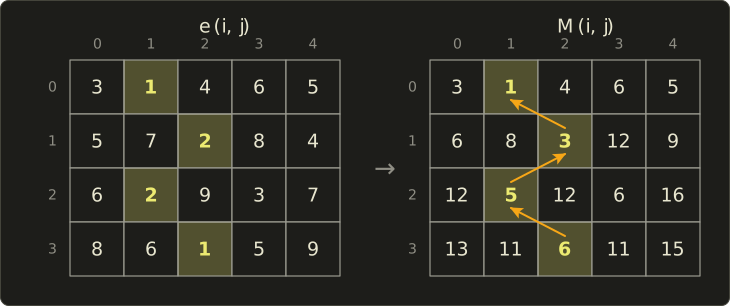
Row 0 is copied.
Row 1, column 2: .
Row 2, column 1: .
Row 3, column 2: .
The minimum of the last row is 6, in column 2.
Going back up: above column 2 the smallest of is in column 1; above that, the smallest of is in column 2; above that, the smallest of is in column 1.
The seam runs through columns 1, 2, 1, 2 with energies .
The cheapest straight column (column 1 or 2) costs 16, so the wiggling seam removes far less important content than cropping out one column would.
In practice
To shrink an image by columns, find and remove the cheapest seam times, recomputing the energy each time; horizontal seams change the height, and duplicating the cheapest seams enlarges the image.
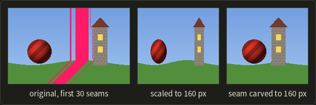
The seams avoid the ball and the tower and run through the sky and the grass, so the objects keep their shapes while the empty space between them shrinks.
It fails when nothing unimportant is left (a crowd), and it bends straight lines that cross many seams; tools let the user protect regions, or force all seams through an object to remove it.
Exam points
- Computational photography = capture several or coded images + computation, to get what one exposure can't.
- HDR merging needs several exposures of a static scene (usually different shutter times), the camera's response curve (linear for RAW, recovered for JPEG, Debevec–Malik 1997) and weights that ignore clipped and very dark pixels; the result is radiance in floating point and needs tone mapping for display.
- Stitching: feature points → matching → homography (8 unknowns, 4 points) with RANSAC → warping → blending. A homography is exact only for a rotating camera or a planar scene.
- Averaging frames divides the noise by .
- Blur is a convolution with the PSF; deconvolution amplifies noise at frequencies the PSF suppresses; coded exposure and coded aperture make the PSF easier to invert.
- Light field cameras trade spatial resolution for directions and allow refocusing after the shot.
- Seam carving removes 8-connected, one-pixel-per-row paths of minimum energy found by dynamic programming.
16.8 Non-photorealistic rendering
Non-photorealistic rendering (ノンフォトリアリスティックレンダリング, NPR) is defined by what it isn't: rendering that doesn't aim to look like a photograph.
The name is a bit unlucky, since it covers very different goals:
- Illustration and communication: technical manuals, patent drawings, medical and scientific illustration, which leave things out on purpose so the important parts read clearly.
- Style: cartoons and anime, comics, paintings, ink drawings, games with a distinctive look.
- Abstraction: reducing a scene or photo to what matters (a map, a sketch).
NPR methods come in two families.
3D (object-based) methods start from a model and have the geometry available: normals, depth, edges, curvature. Toon shading and most line drawing work this way.
2D (image-based) methods start from an image, a photo or a rendered frame, and filter it or place strokes on it: painterly filters, the Kuwahara filter, neural style transfer.
Many systems mix both, like the outlines of section 16.10.
16.9 Toon shading
The idea
Hand-drawn animation (cel animation) colors a character with a few flat tones: a base color, a shadow color, maybe a highlight, with sharp borders between them.
Toon shading (トゥーンシェーディング), also cel shading (セルシェーディング), imitates that by quantizing the diffuse term of section 10.10.
Instead of the smooth , the brightness jumps between a few levels at chosen thresholds.
With two thresholds, 0.2 and 0.6, and three levels:
Note that the darkest level is 0.3, not 0: in a cartoon, the shadow side is a darker version of the color, never black.
Worked example
The light comes from (unit length: ), and the material color is with a white light.
| Normal | Lambert | Toon level | Toon color | |
|---|---|---|---|---|
| 0.8 | (0.64, 0.08, 0.08) | 1.0 | (0.8, 0.1, 0.1) | |
| 0.48 | (0.384, 0.048, 0.048) | 0.6 | (0.48, 0.06, 0.06) | |
| 0.28 | (0.224, 0.028, 0.028) | 0.6 | (0.48, 0.06, 0.06) | |
| 0 | (0, 0, 0) | 0.3 | (0.24, 0.03, 0.03) |
The second and third normals differ in Lambert brightness (0.48 vs 0.28) but get the same toon color: inside a band, the shape information is thrown away on purpose, and only the band borders show the form.
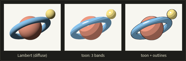
The middle and right images use exactly the thresholds above; the highlight is a fourth "band" where (the half vector of section 10.10) exceeds 0.985, painted white.
Ramp textures
Hard-coded thresholds are hard for artists to tune.
Most engines instead look the level up in a ramp texture (ランプテクスチャ): a 1D texture (a strip of pixels) that the artist paints.
The texture coordinate is , which maps the range −1 to 1 onto 0 to 1.
Example: gives ; in a 256-pixel ramp that's texel .
A ramp can hold any number of bands, soft or hard borders and even a hue shift (a reddish shadow on skin).
// Toon shading: Lambert's n.l quantized into three bands (thresholds 0.2 and 0.6)
float3 toonShade(float3 n, float3 l, float3 baseColor) {
  float nl = dot(normalize(n), normalize(l));
  float level = nl < 0.2 ? 0.3 : (nl < 0.6 ? 0.6 : 1.0);
  return baseColor * level;
}

// The same with an artist-painted ramp texture: u = (n.l + 1) / 2
float3 toonRamp(Texture2D ramp, SamplerState rampSampler, float3 n, float3 l, float3 baseColor) {
  float u = dot(normalize(n), normalize(l)) * 0.5 + 0.5;
  return baseColor * ramp.Sample(rampSampler, float2(u, 0.5)).rgb;
}
// Toon shading: Lambert's n.l quantized into three bands (thresholds 0.2 and 0.6)
vec3 toonShade(vec3 n, vec3 l, vec3 baseColor) {
float nl = dot(normalize(n), normalize(l));
float level = nl < 0.2 ? 0.3 : (nl < 0.6 ? 0.6 : 1.0);
return baseColor * level;
}
// The same with an artist-painted ramp texture: u = (n.l + 1) / 2
vec3 toonRamp(sampler2D ramp, vec3 n, vec3 l, vec3 baseColor) {
float u = dot(normalize(n), normalize(l)) * 0.5 + 0.5;
return baseColor * texture(ramp, vec2(u, 0.5)).rgb;
}// Toon shading: Lambert's n.l quantized into three bands (thresholds 0.2 and 0.6)
float3 toonShade(float3 n, float3 l, float3 baseColor) {
float nl = dot(normalize(n), normalize(l));
float level = nl < 0.2 ? 0.3 : (nl < 0.6 ? 0.6 : 1.0);
return baseColor * level;
}
// The same with an artist-painted ramp texture: u = (n.l + 1) / 2
float3 toonRamp(Texture2D ramp, SamplerState rampSampler, float3 n, float3 l, float3 baseColor) {
float u = dot(normalize(n), normalize(l)) * 0.5 + 0.5;
return baseColor * ramp.Sample(rampSampler, float2(u, 0.5)).rgb;
}Anime-style rendering in games
Sega's Jet Set Radio (2000) is usually credited as the first cel-shaded game; anime-style 3D is now a genre of its own.
A face lit by plain gets shadow shapes no animator would draw, so such games add edited normals that put the shadow borders where a drawing would, per-character lights, textures marking areas always or never in shadow, and sometimes animation that holds each pose for 2 or 3 frames.
16.10 Outlines and line drawing
A few lines are enough to recognize a shape.
A 3D line drawing uses four kinds of edges:
- Silhouette edges (シルエットエッジ, also 輪郭エッジ): where the surface turns away from the viewer. This includes the outer outline and inner contours (where one part of an object passes in front of another).
- Crease edges (クリースエッジ): sharp features of the geometry, where the angle between the two faces is large (the edges of a cube).
- Boundary edges (境界エッジ): the border of an open mesh, an edge with only one face.
- Material or object borders: where the color or the object ID changes.
The silhouette test
Section 11.3 needed silhouette edges as seen from a light; for drawing we need them as seen from the eye.
For a mesh, an edge is a silhouette edge when one of its two faces is front-facing and the other back-facing, with the direction from the edge to the eye:
It's the back-face test of section 10.1, applied to both neighbors of an edge.
For a smooth surface, the silhouette is where exactly.
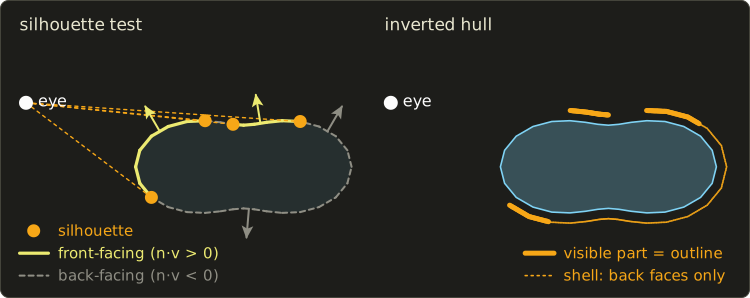
The left half is computed: every edge of the polygon is classified by the sign of , and the silhouette points are where the sign flips.
There are four, not two: the dent on top creates an inner contour, which the eye sees as one hump in front of the other.
Worked example.
Two faces meet at an edge through , with normals and (a wedge pointing in +x).
- Eye at : (it doesn't need to be normalized; only the sign matters). and : a silhouette edge.
- Eye at : , both products are : both faces are visible, not a silhouette.
Is it a crease edge?
The angle between the normals is .
With a crease threshold of 60° (), , so yes: this edge is drawn from every viewpoint, while the silhouette status depends on the eye.
Object-space outlines: the inverted hull
Finding silhouette edges per frame needs the mesh's edge adjacency and work on every edge.
A cheap, very popular trick in games avoids that entirely: the inverted hull method (in Japanese usually 背面法, the "back-face method").
- Make a copy of the mesh, and push every vertex outwards along its normal by a small distance : an enlarged shell.
- Draw the shell in the outline color with front faces culled, so only its back faces are drawn (the opposite of normal back-face culling, which you'll set up in the OpenGL series, chapter 16).
- Draw the object normally. With the depth test, it covers the shell everywhere except in a thin band just outside its silhouettes.
The right half of the figure shows the result: the back faces of the shell are hidden behind the object, except where they stick out beyond a silhouette.
The line width is in world units, so it shrinks with distance.
Example: with m and a focal length of 1000 pixels, an object at 5 m gets an outline of about pixels, at 20 m only 1 pixel; engines often scale with the distance (or do the offset in clip space) to keep a constant width.
It misses creases inside the outline, opens gaps at corners with split normals, and needs a closed mesh.
Image-space outlines: edges in the G-buffer
The other approach renders the scene first and finds the lines in the images.
Takafumi Saito and Tokiichiro Takahashi ("Comprehensible Rendering of 3-D Shapes", SIGGRAPH 1990) introduced the G-buffer (Gバッファ): besides the color, store per pixel the depth, the normal and the object ID, then run 2D edge detection on those buffers.
- A jump in depth marks a silhouette (an object in front of something farther away).
- A jump in the normal marks a crease.
- A change of object ID marks the border between objects.
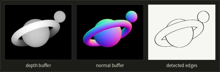
The edge detectors are those of chapter 15, applied to depth and normals instead of colors, which is far more reliable than searching the shaded image, where shadow borders would count as edges too.
The cost doesn't depend on scene complexity, but the widths are in pixels, and thin or distant details can be missed or flicker.
The outlines of the toon picture were made exactly this way; you'll write such a post-processing pass in the OpenGL series, chapter 17.
16.11 Technical illustration: Gooch shading
Technical illustrators keep the shading in the mid-tones, so that black outlines and white highlights stay visible; Phong shading breaks that rule, since its shadow side goes nearly black.
Amy Gooch, Bruce Gooch, Peter Shirley and Elaine Cohen ("A Non-Photorealistic Lighting Model for Automatic Technical Illustration", SIGGRAPH 1998) replaced the dark-to-light change with a cool-to-warm change: Gooch shading (グーチシェーディング).
Surfaces facing the light become warm (yellowish), surfaces facing away cool (bluish), and both stay fairly light; the eye reads the hue shift as shape.
The model mixes two colors, each a fixed tone plus some of the object's own color :
Unlike Lambert, is not clamped at 0: runs from 0 (facing exactly away) to 1 (facing the light), so the side away from the light still has shading.
The paper's figures use values like , , .
Worked example
A red part, , with , , :
| Gooch | Lambert | ||
|---|---|---|---|
| 1 | 1 | (0.88, 0.46, 0.06) | (0.8, 0.1, 0.1) |
| 0.6 | 0.8 | (0.736, 0.372, 0.132) | (0.48, 0.06, 0.06) |
| 0 | 0.5 | (0.52, 0.24, 0.24) | (0, 0, 0) |
| −1 | 0 | (0.16, 0.02, 0.42) | (0, 0, 0) |
For example at : .
Where Lambert gives black for half the object, Gooch shading keeps changing all the way round, from orange to purple-blue.
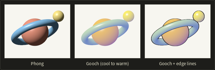
With black silhouette and crease lines (section 16.10) and white highlights added, this is the "illustration" look of many CAD tools.
16.12 Hatching, stippling and painterly styles
Tone from strokes
Pen-and-ink drawings, engravings and comics can't vary the gray of the ink: they make tone with stroke density.
More lines (or dots) per area means darker.
So an NPR renderer first computes a tone per pixel (for example the Lambert brightness), then decides how much ink to put there.
Hatching (ハッチング) uses parallel lines.
With lines of width spaced apart, the inked fraction is ; one layer of 1-pixel lines every 5 pixels gives 20% ink.
For darker tones, add cross-hatching layers in other directions.
The figure uses three layers: diagonal lines where the darkness (1 − tone) exceeds 0.25, the other diagonal above 0.5, horizontal lines above 0.75.
Stippling (点描) uses dots.
To reach a darkness in an area with dots of area , about dots are needed (ignoring overlaps).
Example: a 20 × 20 pixel area with darkness 0.3 and dots of radius 1 pixel ( px²) needs dots.
The figure places one candidate dot at a random position in every 3 × 3 pixel cell and keeps it with probability , so the dot density follows the darkness.
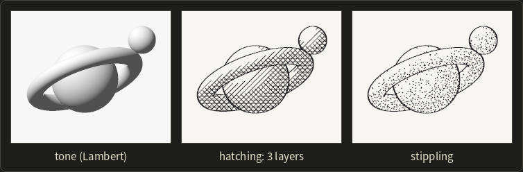
These lines are fixed to the screen, so in motion the object seems to slide behind a fixed pattern (the "shower door" effect).
Real systems attach the strokes to the surface; real-time hatching (Praun, Hoppe, Webb and Finkelstein, SIGGRAPH 2001) uses "tonal art maps", mipmapped hatching textures of increasing darkness, each containing all the strokes of the lighter ones.
Painterly, watercolor and pencil rendering
Painterly rendering (絵画調レンダリング) is stroke-based: it builds an image from many brush strokes with a position, direction, length, color and texture (Haeberli's "Paint by Numbers", SIGGRAPH 1990; Hertzmann's curved strokes of several sizes, large ones first, SIGGRAPH 1998).
Watercolor rendering simulates pigment and water on paper (Curtis et al., SIGGRAPH 1997): dark edges where pigment collects, granulation, bleeding on wet paper.
Pencil rendering combines stroke textures with a paper texture whose grain catches the graphite only on its peaks.
Image-based filters and style transfer
Some NPR filters work on any photo.
The Kuwahara filter (桑原フィルタ; Michiyoshi Kuwahara and colleagues, 1976, first for medical images) looks at four overlapping square regions around each pixel and outputs the mean of the region with the smallest variance.
Flat regions get smoothed, edges stay sharp (the chosen region never straddles an edge), and the result looks like flat patches of paint.
Repeated bilateral filtering (chapter 15), with the lightness quantized into a few levels and edge lines added, gives a similar cartoon-like abstraction of photos and video.
Neural style transfer (Leon Gatys, Alexander Ecker and Matthias Bethge, 2015) uses a convolutional neural network trained for image recognition: it searches for an image whose deep features match the content of one image and whose feature statistics match the style of another (a painting).
Generated "in the style of" images also raise the intellectual property questions of section 18.7.
Exam points
- NPR: rendering that does not aim at photorealism; goals are illustration and communication, style, abstraction. 3D (model-based) vs 2D (image-based) methods.
- Toon (cel) shading quantizes into a few levels by thresholds or a ramp texture; the shadow level is a darker color, not black.
- Silhouette edge of a mesh: one adjacent face front-facing, the other back-facing, ; on a smooth surface . Crease edges are found by the angle between the face normals and don't depend on the viewpoint.
- Inverted hull (背面法): enlarged copy along the normals, drawn with front faces culled. Image-space outlines: edge detection on depth, normal and ID buffers (G-buffer).
- Gooch shading: cool-to-warm blend with , mid-tones only, for technical illustration with black lines and white highlights.
- Hatching and stippling make tone with stroke or dot density: darker = more strokes.
16.13 Visualization: data and goals
Visualization (可視化) turns data into images so that people can see structure, patterns and outliers that would be invisible in a table of numbers.
Two traditions:
- Scientific visualization (科学的可視化): data with a natural position in space and time, from measurements or simulations. A CT scan, the air flow around a car, the temperature in an engine block. The question is mostly "what happens where?".
- Information visualization (情報可視化): abstract data without a natural geometry: sales by region, a social network, a file system, a genome. The designer has to choose the layout.
Scientific data is classified by what is stored at each point:
- Scalar field (スカラー場): one number per point (temperature, density, a CT value).
- Vector field (ベクトル場): a direction and size per point (velocity, a magnetic field).
- Tensor field (テンソル場): a matrix per point (stress in a material; the diffusion tensors of diffusion MRI, which show nerve fiber directions).
and by how the points are arranged:
- Structured grids (構造格子): a regular array, where neighbors are found by index (CT voxels, or a grid wrapped around a wing).
- Unstructured grids (非構造格子): cells of any shape (tetrahedra, hexahedra) with explicit connectivity, typical of finite element simulations.
- Scattered points without any grid (weather stations), which are interpolated first.
The process is often drawn as the visualization pipeline: data → filtering (select, resample) → mapping (to geometry and color) → rendering.
16.14 Scalar fields: color maps, contour lines and isosurfaces
Color maps
The most direct way to show a 2D scalar field is to color each point by its value with a color map (カラーマップ, also called pseudo-coloring).
Three kinds are used:
- Sequential: from low to high, with lightness changing in one direction (density, height).
- Diverging: two hues meeting at a neutral middle (temperature above and below a reference, positive and negative error).
- Qualitative: distinct hues without order, for categories.
For quantities, the key requirement comes from chapter 3: the eye reads order and magnitude mostly from lightness, so the lightness should increase steadily with the value, and equal steps in value should look like equal steps in color.
A map designed in a perceptually uniform space such as CIELAB (section 3.4) can do that; such maps are called perceptually uniform.
The classic rainbow map (blue → cyan → green → yellow → red; "jet" in MATLAB and older Matplotlib) fails this test:
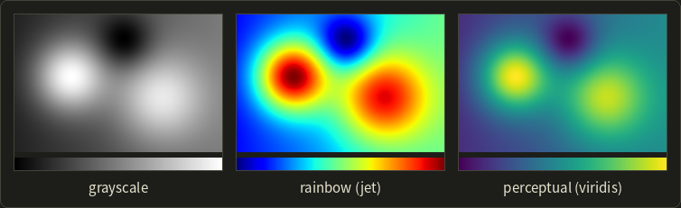
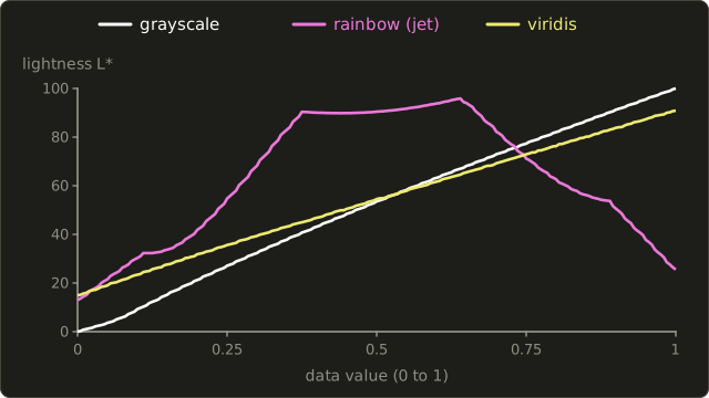
I computed the lightness of each map's colors with the formulas of chapter 3:
| Value | 0 | 0.25 | 0.5 | 0.625 | 0.75 | 1 |
|---|---|---|---|---|---|---|
| jet | 13.0 | 54.7 | 90.5 | 95.2 | 71.2 | 25.5 |
| viridis | 14.9 | 35.7 | 54.5 | 63.6 | 72.9 | 90.9 |
So jet has three problems:
- Not monotonic: its lightness peaks around 0.64 (yellow) and falls again, so the highest values (dark red) are about as dark as low ones (dark blue); in grayscale, high and low look alike.
- Uneven: between 0.37 and 0.64 the lightness hardly changes, while it jumps elsewhere, and sharp hue changes (cyan, yellow) create bands that look like boundaries in a smooth field: the rings in the picture.
- Color vision deficiency: its information relies on red versus green, the most common deficiency of section 3.2.
Visualization researchers have warned about this for a long time ("Rainbow Color Map (Still) Considered Harmful", Borland and Taylor, 2007), and Matplotlib 2.0 (2017) replaced jet with viridis as its default: lightness rises monotonically from about 15 to 91, and it stays readable in grayscale and for most color vision deficiencies.
Distinct hues are fine for categories, but for a continuous quantity, use a perceptually ordered map.
Contour lines and isosurfaces
A contour line or isoline (等値線) connects the points with the same value, like the height contours of a map; drawing several at regular intervals gives a contour plot.
Its 3D version is the isosurface (等値面).
Both are extracted by the marching squares and marching cubes algorithms of section 9.3: classify the grid corners against the iso value, look up the case, interpolate the crossing points along the edges.
An isosurface is an ordinary triangle mesh, fast to display and easy to measure, but it shows one value as an opaque surface: other values are gone, and everything inside is hidden.
16.15 Volume rendering
Direct volume rendering
Volume rendering (ボリュームレンダリング) in the narrow sense, direct volume rendering (DVR), skips the surface and renders the volume itself as a semi-transparent, glowing medium.
It was introduced in 1988, by Marc Levoy ("Display of Surfaces from Volume Data", IEEE Computer Graphics and Applications) and by Robert Drebin, Loren Carpenter and Pat Hanrahan ("Volume Rendering", SIGGRAPH 1988).
The most common method is ray casting (レイキャスティング法) through the volume:
- For each pixel, cast a ray from the eye through the volume.
- Step along the ray at regular intervals and sample the field, interpolating trilinearly between the 8 surrounding voxels (the 3D version of the bilinear interpolation of chapter 11).
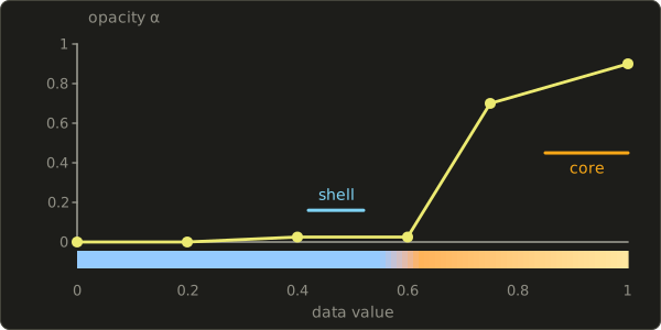
- Classify each sample with the transfer function (伝達関数): it maps the value to a color and an opacity.
- Shade it (optional): use the gradient of the field as a normal and apply a lighting model, so structures look three-dimensional.
- Composite the samples along the ray into the pixel color.
The transfer function
The transfer function decides what is visible.
Values that should disappear get opacity 0; important values get high opacity and a distinct color.
In CT data (Hounsfield units from section 9.3), a typical choice makes air transparent, skin and soft tissue faint and reddish, and bone opaque and white; the same scan with another transfer function can show only the blood vessels filled with contrast agent.
Designing it is the hard part, so programs offer presets and a curve editor:
Front-to-back compositing
Each sample along the ray, nearest first, has a color and an opacity from the transfer function.
It's the over operator of section 10.12, applied to a stack of thin layers.
Going front to back, keep the accumulated color and opacity , both starting at 0:
is the fraction of light from behind that still gets through all the samples in front, so each new sample contributes only through what's left.
At the end, the background is added with the remaining transparency: .
The back-to-front order uses the plain over operator instead, , starting from the background; both give the same result.
Worked example.
Three samples, a red one with , a green one with and a blue one with , in front of a white background:
| After sample | weight | ||
|---|---|---|---|
| 1 (red) | (0.3, 0, 0) | 0.3 | |
| 2 (green) | (0.3, 0.35, 0) | 0.65 | |
| 3 (blue) | (0.3, 0.35, 0.21) | 0.86 |
With the background: .
Check back to front: blue over white gives ; green over that, ; red over that, . The same.
Notice how little the blue sample counts: it is the most opaque, but only 35% of the light still got through the samples in front of it.
Front to back has a big practical advantage: once is close to 1, nothing behind can change the pixel any more, so the ray can stop.
This early ray termination (早期レイ終了) often saves most of the work in dense volumes.
MIP and the comparison
Maximum intensity projection (最大値投影法, MIP) needs no transfer function at all: each pixel shows the largest value along its ray.
It's standard for blood vessels in CT and MR angiography, where the contrast-filled vessels are the brightest structures, but it has no depth cues: a bright structure in front and one behind look the same.
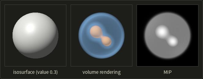
| Isosurface | Direct volume rendering | MIP | |
|---|---|---|---|
| shows | one value as an opaque surface | many values at once, semi-transparent | the maximum along each ray |
| preprocessing | marching cubes, a mesh | none (a transfer function) | none |
| per frame | fast rasterization of triangles | expensive: many samples per pixel | samples per pixel, simple |
| depth impression | good (shading) | good with shading | poor |
| typical use | bone surfaces, measuring, 3D printing | medical and scientific exploration | angiography |
Medical visualization of CT and MRI combines all three with 2D slices (axial, sagittal, coronal).
The emission–absorption model and GPU implementations are in Part 2; ray marching on the GPU appears in the GLSL series, chapter 14.
16.16 Vector fields: glyphs, streamlines and LIC
Glyphs
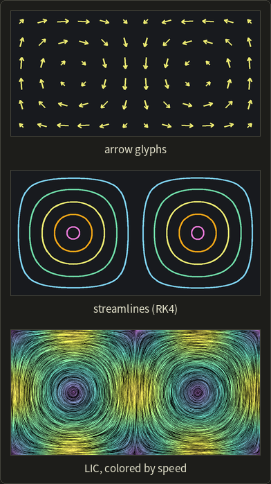
The direct approach draws a small arrow, a glyph (グリフ), at sample points: its direction shows the direction of the field, its length or color the magnitude.
Simple and exact at those points, but arrows clutter quickly and leave the flow between them to guesswork.
Streamlines
A streamline (流線) is a curve that is tangent to the field everywhere: a massless particle released into a steady flow would follow it.
Mathematically it solves the differential equation
starting at a seed point .
It is integrated with the methods of section 14.2, the simplest being the explicit Euler method (陽的オイラー法): step a little along the current direction,
Worked example.
The rotating field has circles around the origin as its exact streamlines.
Start at with :
- , so .
- , so .
- , so .
The distances from the origin are 1, 1.118, 1.25 and 1.398: instead of a circle of radius 1, Euler's method spirals outwards.
Each step moves at right angles to the radius, so the radius grows by the factor per step: after 12 steps, the radius is .
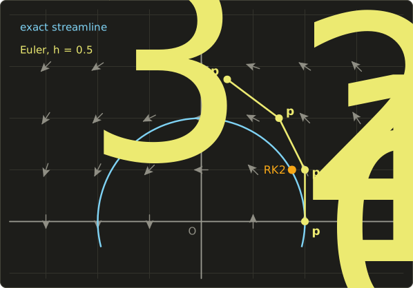
The midpoint method (RK2) of section 14.2 does much better: its half step reaches , where , so , at radius : an error of 0.8% instead of 11.8%.
The fourth-order Runge–Kutta method (RK4) is the usual choice; the streamlines in the figure above used it.
Choosing the seed points is a design problem of its own (too few miss features, too many clutter).
For flows that change over time, streamlines (the field frozen at one instant), pathlines (the path of one particle over time) and streaklines (all particles released from one point, like a line of smoke) differ; in a steady flow they coincide.
Line integral convolution
LIC (line integral convolution, 線積分畳み込み; Brian Cabral and Leith Leedom, SIGGRAPH 1993) shows the whole field at once, at pixel resolution.
Start with an image of white noise.
For each pixel, trace the streamline through it a short distance forward and backward, and set the pixel to the average of the noise along that piece of streamline.
Pixels on the same streamline average nearly the same noise values and get similar brightness, while pixels on neighboring streamlines don't: the result looks like fine brush strokes along the flow, as in the third panel above (which averaged 20 steps of 0.5 pixel in each direction).
LIC shows the direction but not the sense (forward or backward) or the speed, so it's usually combined with a color map of the magnitude.
16.17 Information visualization
Abstract data has no natural positions, so the designer maps the data attributes to visual variables (視覚変数).
Jacques Bertin (Sémiologie graphique, 1967) listed them: position, size, shape, value (lightness), color hue, orientation and texture.
For quantities, position along a common axis and length are read most accurately, area, angle and color much less so (a bar chart beats a pie chart); for categories, hue and shape work well; for order, lightness and size.
Common forms are charts (bar, line, scatter, histogram), networks (node-link diagrams, often laid out by a force-directed simulation of springs and repulsion), hierarchies (trees, and treemaps, ツリーマップ, Ben Shneiderman, 1992, which fill a rectangle with nested rectangles whose areas are proportional to the values) and multidimensional views such as parallel coordinates.
Worked example: a slice-and-dice treemap.
A 10 × 6 rectangle (area 60) shows three items A = 30, B = 18, C = 12, and B contains B1 = 12 and B2 = 6.
Slice the rectangle vertically in proportion to the values: widths , , , all 6 high.
Then dice B (3 wide, 6 high) horizontally: heights and .
Check: and .
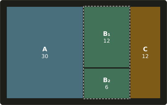
Slice-and-dice is simple but produces long thin rectangles (C is 2 × 6, an aspect ratio of 3), which are hard to compare; "squarified" layouts reorder and group the items to keep the rectangles close to squares.
Visual analytics (ビジュアルアナリティクス) combines interactive visualization ("overview first, zoom and filter, then details on demand", in Shneiderman's words) with automatic analysis by statistics and machine learning.
Honest scales (bars start at zero) and no decorative 3D that distorts lengths and areas are part of the job.
Exam points
- Scientific visualization: data with spatial positions (scalar, vector, tensor fields on structured or unstructured grids). Information visualization: abstract data, layout chosen by the designer.
- Color maps: lightness should increase monotonically with the value; the rainbow map isn't monotonic or uniform, creates false boundaries and depends on red–green discrimination; prefer perceptually uniform maps (viridis) or diverging maps for signed data.
- Isolines and isosurfaces (marching squares and cubes) show one value as a line or opaque surface; direct volume rendering shows many values semi-transparently through a transfer function (value → color, opacity).
- Front-to-back compositing: , ; allows early ray termination; back-to-front with the over operator gives the same result. MIP shows the maximum along each ray, without depth cues.
- Streamlines are tangent to the field; the explicit Euler method drifts (spirals outward in a rotation); Runge–Kutta methods are more accurate. LIC smears noise along streamlines.
- Treemaps show hierarchies as nested rectangles with areas proportional to the values.
16.18 Summary
- Computational photography combines several or coded captures with computation: HDR merging and tone mapping, stitching, focus stacking, light field refocusing, deconvolution, burst denoising (), flash/no-flash, synthetic depth of field, super-resolution, relighting and seam carving.
- NPR aims at illustration, style and abstraction: toon shading quantizes ; lines come from silhouettes, creases and boundaries, in object space (mesh edges, inverted hull) or image space (G-buffer edges); Gooch shading blends cool to warm; hatching and stippling make tone from stroke density; painterly filters and style transfer work on images.
- Visualization maps scalar, vector and tensor fields (scientific) or abstract data (information) to images: perceptually ordered color maps, isosurfaces, direct volume rendering with transfer functions and compositing, MIP, glyphs, streamlines, LIC, charts, networks and treemaps.
16.19 Key terms
| English | 日本語 |
|---|---|
| computational photography | コンピュテーショナルフォトグラフィ |
| dynamic range | ダイナミックレンジ |
| exposure bracketing | 露出ブラケット |
| HDR image | ハイダイナミックレンジ画像(HDR画像) |
| response curve | 応答曲線 |
| tone mapping | トーンマッピング |
| image stitching | 画像のスティッチング |
| feature point | 特徴点 |
| homography | ホモグラフィ |
| focus stacking | 深度合成(フォーカススタッキング) |
| light field camera | ライトフィールドカメラ |
| refocusing | リフォーカス |
| point spread function (PSF) | 点像分布関数(PSF) |
| deconvolution | 逆畳み込み(デコンボリューション) |
| coded exposure | 符号化露光 |
| coded aperture | 符号化開口 |
| burst photography | バースト撮影 |
| super-resolution | 超解像 |
| image-based relighting | イメージベーストリライティング |
| seam carving | シームカービング |
| seam | シーム |
| dynamic programming | 動的計画法 |
| non-photorealistic rendering (NPR) | ノンフォトリアリスティックレンダリング(NPR) |
| toon shading, cel shading | トゥーンシェーディング、セルシェーディング |
| ramp texture | ランプテクスチャ |
| silhouette edge | シルエットエッジ(輪郭エッジ) |
| crease edge | クリースエッジ |
| inverted hull | 背面法 |
| G-buffer | Gバッファ |
| Gooch shading | グーチシェーディング |
| hatching | ハッチング |
| stippling | 点描 |
| painterly rendering | 絵画調レンダリング |
| Kuwahara filter | 桑原フィルタ |
| visualization | 可視化 |
| scientific visualization | 科学的可視化 |
| information visualization | 情報可視化 |
| scalar field, vector field, tensor field | スカラー場、ベクトル場、テンソル場 |
| structured grid, unstructured grid | 構造格子、非構造格子 |
| color map | カラーマップ |
| isoline (contour line) | 等値線 |
| isosurface | 等値面 |
| volume rendering | ボリュームレンダリング |
| transfer function | 伝達関数 |
| early ray termination | 早期レイ終了 |
| maximum intensity projection (MIP) | 最大値投影法(MIP) |
| glyph | グリフ |
| streamline | 流線 |
| explicit Euler method | 陽的オイラー法(前進オイラー法) |
| line integral convolution (LIC) | 線積分畳み込み(LIC) |
| visual variables | 視覚変数 |
| treemap | ツリーマップ |
| visual analytics | ビジュアルアナリティクス |
16.20 Challenges
- ★ A camera with a linear response takes three shots of a scene at , and s. One pixel reads , 200 and 52. Compute the radiance estimate and the hat weight of each shot, and merge them with the weighted average of logarithms of section 16.2. What does the first shot tell you about the radiance?
- ★★ Find the cheapest vertical seam of the energy table with rows (4, 2, 5, 7), (6, 3, 1, 8), (2, 9, 5, 3), (7, 1, 6, 5) by filling the table . Give its columns and cost, and compare with the cheapest straight column.
- ★★ A green part with is lit from . For the normals , and , compute the toon color with the thresholds 0.2 and 0.6 of section 16.9, and the Gooch color with , , . Which of the three points would Lambert shading show as black?
- ★★ Trace the streamline of from to with Euler's method, once with and once with . The exact streamline is : compare the errors at . What does halving the step do to the error?
- ★★★ For a CT scan of a head, sketch a transfer function (opacity and color against the Hounsfield value) that shows the skull opaque and the skin faint. Explain why one isosurface can't show both, what MIP would show, and why a rainbow color map is a poor choice for a 2D slice.
Multiple choice
Q1 ★ Which of the following statements about creating an HDR image from bracketed exposures is correct?
| A | Each exposure gives an estimate of the radiance from its linearized pixel value divided by its exposure time, and clipped or very dark pixels get little or no weight in the merge. |
| B | All exposures of the bracket must use the same shutter speed; only the aperture is changed between them. |
| C | The merged HDR image can be shown directly on an ordinary 8-bit display, without tone mapping. |
| D | The camera's response curve never matters, because every camera stores pixel values proportional to the light. |
| E | Objects that move between the exposures cause no problems, because each pixel is merged independently. |
Q2 ★ Which of the following statements about NPR techniques is correct?
| A | Toon shading evaluates the specular highlight per pixel and blurs it to produce smooth gradients. |
| B | In Gooch shading, the side of an object facing away from the light is drawn black so that it contrasts with the outlines. |
| C | An edge of a closed mesh is a silhouette edge when one of its two faces is front-facing and the other back-facing as seen from the eye. |
| D | The inverted hull method draws the enlarged copy of the mesh with its back faces culled. |
| E | Hatching draws more strokes where the surface is brighter. |
Q3 ★★ In direct volume rendering, a ray meets two samples, front to back: the first has intensity 1.0 and opacity 0.4, the second has intensity 0.6 and opacity 0.5. Using front-to-back compositing, starting from and (background not yet added), what are the accumulated intensity and opacity ?
| A | , |
| B | , |
| C | , |
| D | , |
| E | , |
16.21 Practical assignment
Carve, shade and composite on graph paper.
You need graph paper, a ruler, a compass, colored pencils and a calculator.
You'll do one small task from each part of the chapter by hand: resize an image with seam carving, toon-shade a sphere, and render one ray of a volume.
Part A: seam carving.
Here is a 5 × 6 grayscale image (0 = black, 9 = white); the bright 8s and 9s are an object:
| row | col 0 | col 1 | col 2 | col 3 | col 4 | col 5 |
|---|---|---|---|---|---|---|
| 0 | 1 | 1 | 3 | 8 | 9 | 1 |
| 1 | 2 | 1 | 2 | 8 | 9 | 1 |
| 2 | 1 | 3 | 2 | 8 | 9 | 2 |
| 3 | 1 | 3 | 3 | 8 | 9 | 3 |
| 4 | 3 | 1 | 1 | 1 | 3 | 1 |
- Energy. Use the simplified energy (the horizontal difference only), and at the left and right borders use the pixel itself in place of the missing neighbor. Write the 5 × 6 energy table.
- Dynamic programming. Fill the table row by row and find the cheapest seam by walking back from the smallest value of the last row.
- Carve. Remove the seam's pixel from every row and write the new 5 × 5 image. Color the object's pixels.
- Compare. Compute the energy sum of every straight column, and say what scaling the image to 5 columns would do to the object.
Part B: toon shading a sphere.
Draw a circle of radius cm: a sphere seen from the front (orthographic view, ).
A point of the disk at has the normal .
The light comes from .
- Along the horizontal diameter. For cm (so ) and , compute , the Lambert value and the toon level with the thresholds 0.2 and 0.6 of section 16.9. Mark where the band borders cross the diameter.
- The band borders. The points with project to an ellipse with center , vertical semi-axis and horizontal semi-axis . Draw it for . For only its left part is on the visible half: draw it from the diameter to the outline at . Color the three bands.
- The silhouette. Where is on your drawing? Go over that line with a thick black pencil.
Part C: one ray through a volume.
A ray meets four samples, front to back, with the values 0.1, 0.45, 0.8 and 0.5.
The transfer function gives intensity 0 and opacity 0 for values below 0.3, intensity 0.5 and opacity 0.2 for values from 0.3 to 0.6, and intensity 1.0 and opacity 0.7 above 0.6.
The background is black.
- Front to back. Make a table like the one in section 16.15 and composite the four samples. Then stop the ray as soon as (early ray termination) and note how much the result changes.
- Back to front. Composite the same samples with the over operator, starting from the black background.
- Other renderings. What does MIP show for this ray? Where along the ray (in sample units, linearly interpolated) would an isosurface with the value 0.6 be hit?
How to check yourself:
- Part A: the seam has exactly one pixel per row and moves by at most one column from row to row; its cost is 3, less than half of the cheapest straight column (7); the object keeps its full width of two columns in the carved image.
- Part B: reaches its maximum 1 at cm, where ; along the diameter the borders lie at () and (), and the ellipse for touches the outline at . The silhouette is the circle itself.
- Part C: never decreases and never exceeds 1; the front-to-back and back-to-front results agree (0.684); with early termination the pixel comes out a little darker (0.66). MIP shows 0.8, and the isosurface lies between the second and third samples.
コメント(0)
まだコメントはありません。
ログインするとコメント出来ます。