28. Volume Rendering and Advanced NPR
This chapter has two halves.
The first half is volume rendering: fog, smoke, clouds, the sky, and medical scans, where light is absorbed and scattered by the space itself.
The second half is advanced non-photorealistic rendering: anime-style characters, line drawings, hatching, watercolor and image filters, where we decide on purpose what the picture should look like.
Both halves keep promises from Part 1.
Chapter 12 (section 12.6) introduced participating media and the Beer–Lambert law, and said volume rendering would come later.
Chapter 16 showed volume visualization (section 16.15) and promised the emission–absorption model and GPU volume rendering; its NPR sections (16.8 to 16.12) are where the second half starts.
Chapter 9 (section 9.3) gave us voxels and CT data, and I'll link back instead of repeating any of it.
This is Part 2 material and goes beyond the exam syllabus, but it deepens three of its items: photorealistic rendering (写実的表現法, the participating media of chapter 12), and visualization (可視化) and non-photorealistic rendering (ノンフォトリアリスティックレンダリング) from chapter 16.
We'll also use Monte Carlo sampling from chapter 23, and the volume rendering integral of this chapter is exactly what NeRF uses in chapter 29.
28.1 Light in a participating medium
Four things that can happen
A ray of light crossing fog meets tiny particles or molecules.
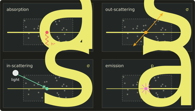
At each of them, one of four things can change the radiance traveling along the ray:
- Absorption (吸収): the light is turned into heat and is gone. The ray gets darker.
- Out-scattering (外向き散乱): the light bounces off in another direction. The ray gets darker, but the light isn't lost; it continues elsewhere.
- In-scattering (内向き散乱): light that was traveling in other directions bounces into the ray. The ray gets brighter. This is why fog glows around a street lamp.
- Emission (放射, 発光): the medium itself produces light, like a flame, an explosion or hot gas. The ray gets brighter.
Coefficients
How often these events happen is described by coefficients with the unit "per meter":
- the absorption coefficient (吸収係数) ,
- the scattering coefficient (散乱係数) ,
- the extinction coefficient (消散係数, also 減衰係数) , which counts everything that removes light from the ray.
Read as a probability per unit length: over a very short distance , the light interacts with probability .
Two derived numbers describe a medium at a glance.
The single-scattering albedo (散乱アルベド) is the fraction of interactions that are scattering rather than absorption: near 1 for clouds and snow-white fog, near 0 for soot.
The mean free path (平均自由行程) is the average distance between interactions.
Example.
A fog with and per meter has per meter, an albedo of and a mean free path of 10 m.
In general the coefficients change from point to point (a smoke plume from the simulation of chapter 26 is a heterogeneous medium, 非一様な媒質) and with the wavelength, which renderers handle by storing one value per RGB channel.
In a homogeneous medium (一様な媒質) they are the same everywhere.
28.2 Transmittance and the Beer–Lambert law
The derivation
Follow a ray through a medium with only extinction (no light added).
Over a short distance , the fraction of the light is removed, so
The rate of loss is proportional to what is left: that is the equation of exponential decay.
Its solution over a path from 0 to is
is the transmittance (透過率), the fraction of light that survives, and is the optical depth (光学的厚さ), the extinction added up along the path.
For a homogeneous medium , and we get back the Beer–Lambert law (ランベルト・ベールの法則) of section 12.6.
Worked example
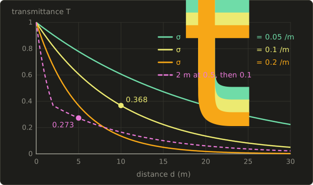
In the fog above ( per meter), and , as in chapter 12.
Now a two-layer medium: 2 m of thick smoke with , then 3 m of the thin fog with :
The same number comes out layer by layer: .
Optical depths add, so transmittances multiply.
That property is what every ray marcher in this chapter uses: it keeps one running transmittance and multiplies it by the transmittance of each small step.
Colored absorption
With one coefficient per channel, transmittance tints the light.
Pure water absorbs red far more than blue; rough values are 0.3 per meter for red, 0.06 for green and 0.01 for blue.
After 10 m of water the transmittances are , and : deep water looks blue-green, and the deeper you dive, the more the reds disappear.
The tint of deep water mentioned in chapter 26 is exactly this.
28.3 The volume rendering integral
The radiative transfer equation
Now let all four events happen.
Along a ray, in a short distance , absorption and out-scattering remove , emission adds , and in-scattering adds :
is the emitted radiance, the radiance arriving at the point from direction , and the phase function (section 28.4), which says how much of the light from is scattered into .
The integral runs over the whole sphere of directions , because a point inside a medium can receive light from everywhere, not only from a hemisphere as on a surface.
This is the radiative transfer equation (放射伝達方程式, RTE), studied in astrophysics long before graphics (Subrahmanyan Chandrasekhar's book Radiative Transfer, 1950).
Integrating along a camera ray
Solving the equation along a camera ray that starts at the eye and hits a surface (or the background) at distance gives the volume rendering integral (ボリュームレンダリング積分):
The surface behind the medium contributes its radiance, dimmed by the transmittance of the whole path; every point in between adds the light it emits or scatters toward us, dimmed by the transmittance between it and the eye.
Chapter 12's "exponential fog" is the special case of a homogeneous medium whose in-scattered light is a constant fog color.
James Kajiya and Brian Von Herzen brought it to graphics ("Ray Tracing Volume Densities", SIGGRAPH 1984), rendering clouds with single scattering.
Nelson Max's survey "Optical Models for Direct Volume Rendering" (IEEE Transactions on Visualization and Computer Graphics, 1995) ordered the simplifications into a ladder: absorption only, emission only, emission plus absorption, single scattering with shadows, multiple scattering.
The emission–absorption model
Direct volume rendering in medicine and science (chapter 16) uses the third rung, the emission–absorption model (放射・吸収モデル).
It drops scattering: every point glows with a color and blocks light with an extinction , both chosen by the transfer function:
There are no light sources and no shadows, so it isn't physical, but it's fast, and a clear way to see inside data.
From the integral to compositing
Split the ray into segments of length and assume and are constant on segment .
If is the transmittance from the eye to the start of the segment, the segment contributes
and the transmittance after it is .
With , that is exactly the front-to-back compositing of section 16.15: , .
So the opacity of a sample is not a free parameter: it is the extinction of one segment, .
Worked example.
Three segments of length have and :
| Segment | weight | after | ||
|---|---|---|---|---|
| 1 | 1 | 0.1813 | 0.1813 | |
| 2 | 0.8187 | 0.5175 | ||
| 3 | 0.3012 | 0.1185 |
The final transmittance is , and it agrees with the Beer–Lambert law for the whole ray: .
Opacity correction
Transfer functions are usually designed as opacities for one reference step (often one voxel).
If the renderer takes a different step , it must convert, since :
Example: per voxel, step half a voxel: .
Two such half steps give , the same as one full step.
Without the correction, two half steps of would give : the volume would look denser just because you sampled it more finely.
28.4 Phase functions
What a phase function says
When light scatters, where does it go?
The phase function (位相関数) is the probability density, per steradian, that light arriving with direction leaves with direction .
It plays the role of the BRDF for a medium, with two differences: it covers the whole sphere, and it is normalized, , because absorption is already handled by .
In fog, smoke or air the particles have random orientations, so depends only on the scattering angle (散乱角) between the incoming direction of travel and the outgoing direction: means straight on, straight back.
- Isotropic (等方的): in every direction.
- Rayleigh (for molecules, section 12.6): . Forward and backward are equal (), sideways is half ().
- Mie scattering by droplets and dust is strongly peaked forward; the exact Mie functions are spiky and expensive, so renderers use a smooth model.
The Henyey–Greenstein phase function
The standard smooth model comes from astronomy: Louis Henyey and Jesse Greenstein proposed it for light scattered by interstellar dust ("Diffuse Radiation in the Galaxy", Astrophysical Journal, 1941):
The single parameter , the asymmetry parameter (非対称パラメータ), is the average of over the scattered light: is isotropic, scatters forward, backward.
Cloud droplets have around 0.85; atmospheric haze is often modeled with .
Worked example: .
At the denominator is , so .
At : .
At : .
Forward beats backward by .
I integrated it numerically for several values of : the total is 1 every time, the mean cosine equals , and for , 94.9% of the scattered light goes into the forward hemisphere.
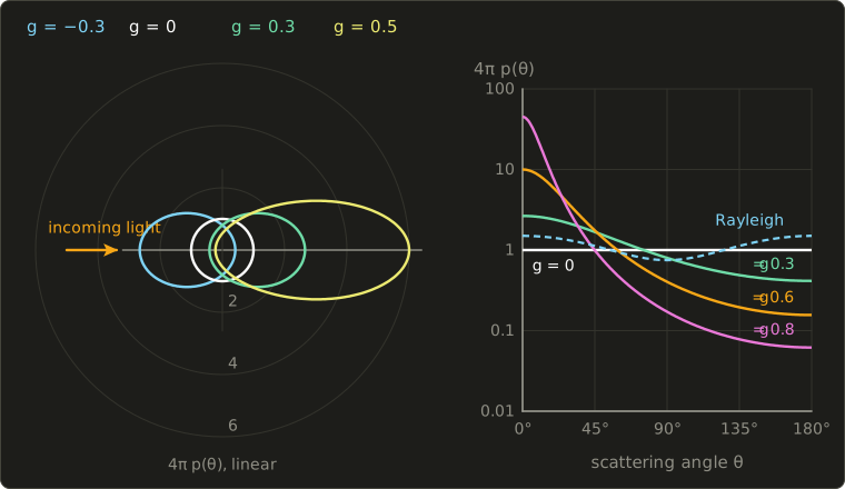
The plots show , so that isotropic scattering is the value 1.
Forward scattering is why a cloud's edge lights up when the sun is behind it (the "silver lining").
Sampling HG
A path tracer needs to draw scattering directions with this density.
The inversion method of chapter 23 gives a closed form: for a uniform random number ,
with the azimuth drawn uniformly around the incoming direction.
Example: , : , so and .
Since is the median, half of all scattered light stays within 19.3° of straight ahead.
Real media are often fit with a mix of two HG lobes, for example : a forward lobe for the silver lining plus some backscatter so the sunlit side isn't flat.
A weighted mix of normalized functions with weights summing to 1 is still normalized.
28.5 Ray marching with single scattering
Single scattering
The in-scattering term needs the light arriving at every point from every direction, which itself depends on the medium everywhere: the full problem is as hard as global illumination.
The first big simplification is single scattering (単一散乱): only light that comes straight from the light source and scatters once toward the camera.
For a directional light such as the sun, with intensity arriving along direction , the in-scattered term becomes
where is the transmittance from the point toward the light: the medium's self-shadowing.
It's found by a second, shorter march toward the light (a "shadow ray"), or read from a shadow map or a precomputed shadow volume.
The algorithm
Ray marching (レイマーチング) evaluates the volume rendering integral by stepping along the ray (the distance-field ray marching of the GLSL series, chapter 14 is a relative that steps toward a surface instead):
- Intersect the ray with the medium's bounding box to get .
- Choose a step and start at plus a random fraction of a step (jitter).
- At each step, look up and , compute , and the source .
- Add the step's contribution to , then multiply the running transmittance by .
- Stop when is tiny (say below 0.01; that's early ray termination, section 16.15) or the ray leaves the box, and add .
The step's contribution, done right
The obvious contribution of step is (a Riemann sum).
But inside the step the transmittance keeps falling, and with large steps or dense media the Riemann sum overestimates.
Sébastien Hillaire ("Physically Based and Unified Volumetric Rendering in Frostbite", SIGGRAPH 2015 Advances in Real-Time Rendering course) popularized the energy-conserving version, which integrates the decay inside the step exactly, as in section 28.3:
Worked example.
A light shaft in the fog of section 28.1 (, , per meter), 20 m long.
The light reaches every point unattenuated with , the phase function is HG with , and the scattering angle is 30°:
Since is constant, the integral has a closed form:
With 4 steps of 5 m, the Riemann sum uses the transmittances 1, 0.6065, 0.3679 and 0.2231 at the step starts: , 27% too bright.
The energy-conserving step gives 1.735 exactly, for any number of steps, because in a homogeneous medium its assumption (constant and within a step) is true.
In a heterogeneous medium it's no longer exact, but it converges much faster and never adds more light than the step can scatter.
In code
The C++ program below compares the two (it uses Vec3, dot and normalize from the Linear Algebra series' linalg.hh):
#include <cmath>
#include <cstdio>
#include <initializer_list>
#include "linalg.hh"

constexpr float kPi = 3.14159265f;

// Henyey-Greenstein: cosTheta = cosine of the angle between the light's direction of travel
// and the scattered direction (1 = straight on, -1 = straight back)
float phaseHG(float cosTheta, float g) {
  float d = 1.0f + g * g - 2.0f * g * cosTheta;
  return (1.0f - g * g) / (4.0f * kPi * d * std::sqrt(d));
}

// Single scattering along one camera ray through a homogeneous medium of length dist.
// The light reaches every point unattenuated (a "light shaft"), so the exact answer is known.
struct Medium { float sigmaS, sigmaA; };

float marchNaive(Medium m, float source, float dist, int steps) {
  float sigmaT = m.sigmaS + m.sigmaA, dt = dist / steps, T = 1.0f, L = 0.0f;
  for (int i = 0; i < steps; ++i) {
    L += T * source * dt;          // Riemann sum: S times the transmittance at the step's start
    T *= std::exp(-sigmaT * dt);
  }
  return L;
}

float marchEnergyConserving(Medium m, float source, float dist, int steps) {
  float sigmaT = m.sigmaS + m.sigmaA, dt = dist / steps, T = 1.0f, L = 0.0f;
  for (int i = 0; i < steps; ++i) {
    float stepT = std::exp(-sigmaT * dt);
    L += T * source * (1.0f - stepT) / sigmaT;   // integral of S e^(-sigmaT s) over the step
    T *= stepT;
  }
  return L;
}

int main() {
  Medium fog{0.08f, 0.02f};                        // per meter
  Vec3 lightTravel = normalize(Vec3{0.0f, -0.5f, -std::sqrt(3.0f) / 2.0f});
  Vec3 toCamera = {0.0f, 0.0f, -1.0f};             // scattered toward the camera
  float cosTheta = dot(lightTravel, toCamera);     // cos 30 degrees
  float E = 10.0f;                                  // light arriving at each point
  float source = fog.sigmaS * phaseHG(cosTheta, 0.5f) * E;
  float sigmaT = fog.sigmaS + fog.sigmaA, dist = 20.0f;
  float exact = source * (1.0f - std::exp(-sigmaT * dist)) / sigmaT;
  std::printf("cos theta = %.4f, p = %.4f, S = %.4f, exact L = %.4f\n",
              cosTheta, phaseHG(cosTheta, 0.5f), source, exact);
  for (int steps : {1, 4, 16, 64})
    std::printf("%3d steps: naive %.4f   energy-conserving %.4f\n", steps,
                marchNaive(fog, source, dist, steps),
                marchEnergyConserving(fog, source, dist, steps));
}
cos theta = 0.8660, p = 0.2508, S = 0.2007, exact L = 1.7351
  1 steps: naive 4.0134   energy-conserving 1.7351
  4 steps: naive 2.2049   energy-conserving 1.7351
 16 steps: naive 1.8458   energy-conserving 1.7351
 64 steps: naive 1.7624   energy-conserving 1.7351
The naive sum needs 64 steps to get within 2%.
Step size, jitter and cost
Any fixed step pattern samples the medium at the same depths in every pixel, which shows up as banding: contour-like stripes in smooth gradients.
Offsetting each pixel's start by a random fraction of a step (different every frame) turns the banding into fine noise, which temporal anti-aliasing (section 20.6) then averages away.
The cost adds up quickly (section 28.9 counts it for clouds: hundreds of millions of density lookups per frame), so real-time renderers march at reduced resolution, reuse previous frames, and precompute the light transmittance into a 3D texture where they can.
A cloud, four ways
Here is a procedural cloud (blobs eroded by 3D noise) ray marched with the method above, the sun behind it and to the upper right:
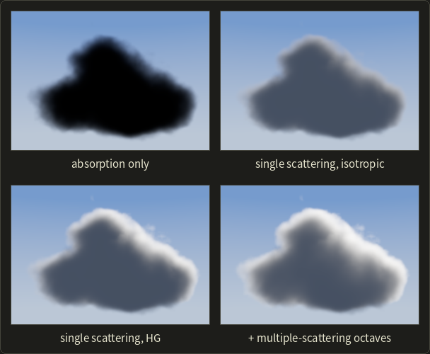
Absorption alone gives a dark smoke stain; isotropic single scattering lights the cloud evenly and dully; the two-lobe HG mix makes the thin edges facing the sun glow; the last image adds the multiple-scattering approximation of the next section.
The light transmittance was precomputed into a shadow volume by marching from every grid point toward the sun.
28.6 Multiple scattering and unbiased tracking
Why single scattering isn't enough for clouds
In a cloud the albedo is almost 1 and the optical depths are large, so light scatters many times before it leaves.
With , the fraction of energy still around after 100 scattering events is : most of it is still there.
Single scattering throws all of that away, so its clouds have dark gray interiors where real clouds are bright white.
An artist-friendly approximation
Magnus Wrenninge, Christopher Kulla and Viktor Lundqvist ("Oz: The Great and Volumetric", SIGGRAPH 2013 talk) approximate multiple scattering by adding octaves of single scattering, each one weaker, but less shadowed and with a rounder phase function:
Their defaults are and .
The idea: light that has scattered many times has "forgotten" its direction (rounder phase), and it reaches deep points by many paths, which acts like a thinner shadowing medium.
Example.
A point deep in a cloud has optical depth toward the sun.
Octave 0 gets the transmittance ; octave 1 gets weight 0.5 and , so 0.0677; octave 2 gets .
Ignoring the phase function, three octaves give , almost 10 times the single-scattering value: the interior lights up, as in the fourth cloud image.
Unbiased methods: free-flight sampling and delta tracking
Film renderers want the correct answer, so they path trace the volume (chapter 23): a path flies through the medium, randomly collides, scatters in a direction drawn from the phase function, and so on.
In a homogeneous medium the distance to the next collision has the density and is drawn by inversion as , as chapter 23 showed.
In a heterogeneous medium there is no closed form, because the optical depth must be integrated.
Delta tracking (デルタトラッキング), also called Woodcock tracking, solves this with a trick from nuclear physics (E. R. Woodcock and colleagues, 1965, for neutron transport in reactors).
Fill the medium with imaginary particles that do nothing, so that the total density becomes a constant majorant (優関数, メジャラント) everywhere.
Collisions with the imaginary particles are null collisions (ヌル衝突): the path just continues.
- Draw a tentative distance and move forward by it.
- If the path left the medium, stop.
- Otherwise accept a real collision with probability ; on a null collision, go to step 1.
It's unbiased: the real collisions land exactly where the true heterogeneous medium would put them, and the only cost of a loose majorant is more null collisions.
Worked example.
A ray of length 2 crosses on and on , with majorant .
The random numbers give steps , so tentative collisions at , and then 2.096, outside.
At the acceptance probability is ; a second random number 0.6 makes it a null collision.
At , a second random number 0.1 is below 0.25: a real collision, where the path would scatter or be absorbed.
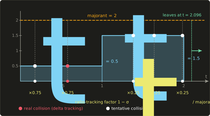
For shadow rays we only need the transmittance, not a collision point.
Ratio tracking (比率トラッキング; Jan Novák, Andrea Selle and Wojciech Jarosz, "Residual Ratio Tracking for Estimating Attenuation in Participating Media", SIGGRAPH Asia 2014) walks the same tentative collisions to the end of the ray and multiplies by at each one.
For the walk above: .
One walk is a noisy estimate, but its average is right: I ran 200,000 walks and got 0.1346 by ratio tracking and 0.1351 as the fraction of delta-tracking paths that escaped, against the exact .
The expected number of tentative collisions is , so production renderers store majorants per region of a coarse grid to keep tight.
28.7 Sky and atmosphere
The model
Section 12.6 explained the blue sky with Rayleigh's .
A renderable atmosphere adds numbers.
Sébastien Hillaire ("A Scalable and Production Ready Sky and Atmosphere Rendering Technique", EGSR 2020) uses, for the Earth:
| Component | Scattering (per m) | Absorption (per m) | Density with altitude | Phase |
|---|---|---|---|---|
| Rayleigh (molecules) | 0 | about | Rayleigh | |
| Mie (aerosols) | about | HG, | ||
| Ozone | 0 | a layer around 25 km | none |
(The scale heights of 8 km for molecules and 1.2 km for aerosols are the classic values, as in Eric Bruneton and Fabrice Neyret's "Precomputed Atmospheric Scattering", 2008.)
The three Rayleigh values follow exactly for wavelengths of 680, 550 and 440 nm: .
Worked example: why the setting sun is red
For an exponential density, the optical depth straight up is : the whole atmosphere acts like a layer of sea-level air 8 km thick.
For Rayleigh scattering alone:
| Channel | up | up | at the horizon | at the horizon |
|---|---|---|---|---|
| red | 0.0464 | 0.955 | 1.64 | 0.194 |
| green | 0.108 | 0.897 | 3.84 | 0.0216 |
| blue | 0.265 | 0.767 | 9.37 | 0.0000856 |
The horizon column needs the path length.
A horizontal ray climbs as on a planet of radius , so : 35.4 times the vertical value (a numerical integration on the real sphere gives the same).
At noon the sun loses about a quarter of its blue; at the horizon, blue is cut to less than a ten-thousandth while red keeps 19%: compared with sunlight outside the atmosphere, red is now 2,262 times stronger than blue.
Rendering the sky
Tomoyuki Nishita and colleagues rendered the Earth's atmosphere with single scattering ("Display of the Earth Taking into Account Atmospheric Scattering", SIGGRAPH 1993).
Bruneton and Neyret precomputed multiple scattering into 4D tables, which made physically based skies usable in real time.
Hillaire's 2020 method recomputes small tables every frame, even on mobile: a transmittance table of 256 × 64, a 32 × 32 multiple-scattering table, a 200 × 100 sky-view table and a 32 × 32 × 32 froxel volume (section 28.8) for aerial perspective (空気遠近法), the haze that makes distant mountains bluish and low in contrast.
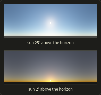
I ray marched every view ray (40 steps, with a 12-step light march at each) using the table's values.
With the sun high, the sky is blue with a white Mie glow around the sun; with the sun low, the light reaching the air near the horizon has lost its blue and turns orange.
Ozone matters at twilight: it absorbs mostly green and red (look at its coefficients), which keeps the sky overhead from turning gray.
28.8 Volumetric fog in games: froxels
The problem
A game wants fog lit by dozens of lights, with shadows, light shafts through windows, local fog volumes, and transparent objects that are fogged correctly.
Marching every pixel through every light is far too expensive.
Frustum-aligned voxels
Bart Wronski ("Volumetric Fog: Unified, Compute Shader Based Solution to Atmospheric Scattering", SIGGRAPH 2014 Advances in Real-Time Rendering course, from Assassin's Creed IV: Black Flag) moved the work into a 3D texture aligned with the view frustum: x and y follow the screen in coarse tiles, z follows depth in slices.
Its cells are called froxels (フロクセル, "frustum voxels").
The game used 160 × 90 × 64 (or 128 slices, depending on the platform), about as many cells as a 720p image has pixels.
The algorithm runs as compute shaders (GLSL series, chapter 15):
- Inject the medium: for each froxel, compute and from global fog, height fog, animated noise and (in later engines) local fog volumes.
- Light each froxel: sum over lights of , with the visibility from shadow maps.
- Integrate front to back along each column of froxels, storing for every froxel the in-scattered light accumulated from the camera to it and the transmittance so far.
- Apply: every pixel (opaque or transparent) looks up the volume at its own depth and computes , one 3D texture fetch and a multiply-add.
Hillaire's 2015 Frostbite talk (section 28.5) made it physically based and unified: all fog, volumes and particles share scattering, absorption, phase and emission parameters, the integration is energy conserving, and froxels are sampled at jittered positions and blended over frames, as in TAA.
At the time of writing, froxel-based volumetric fog is standard in large engines.
Exponential slices
Near the camera the fog must be detailed; far away a few meters per slice is enough.
So the slices are distributed exponentially between the near distance and the far distance :
Example: m, m, slices.
Each slice is times as deep as the one before.
The first slice ends at 1.079 m (7.9 cm thick); slices 16, 32 and 48 end at 3.36 m, 11.31 m and 38.05 m; the last one spans 118.65 m to 128 m (9.35 m thick).
Memory: froxels; at 8 bytes each (four 16-bit floats) that's 7.4 MB per volume, and a renderer keeps a few (medium properties, lit, integrated, the previous frame).
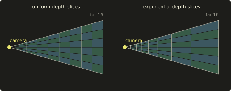
The figure uses , and 8 slices so the near slices stay visible: the exponential slices are 1.414 times deeper each time (1, 1.41, 2, 2.83, 4, …, 16), and the froxels keep a similar shape from near to far.
The price of the low resolution is blur and light leaking through thin walls.
28.9 Clouds
Clouds are too large for froxels and too detailed for a coarse grid, so games ray march them directly.
Andrew Schneider and Nathan Vos ("The Real-time Volumetric Cloudscapes of Horizon Zero Dawn", SIGGRAPH 2015 Advances in Real-Time Rendering course) described a design that many games followed:
- Shape: a 2D weather map (coverage, precipitation, cloud type) and a height gradient per cloud type, eroded by 3D noise: a "Perlin–Worley" texture (Perlin noise dilated by inverted Worley noise) and a Worley texture for detail (noise is in the GLSL series, chapter 8).
- Lighting: Beer's law, Henyey–Greenstein for the silver lining, and a "powder" term that darkens edges facing the light, with 6 light samples in a cone toward the sun.
- Cost: 64 view samples, rising to 128 toward the horizon; one pixel in each 4 × 4 block updated per frame, the rest reprojected; about 2 ms, down from about 20 ms.
Example.
With 64 view samples and 6 light samples each, a 1920 × 1080 frame needs million density samples; updating one pixel in 16 brings that to 58 million.
Film goes the other way: clouds and smoke are stored as sparse voxel grids (OpenVDB, Ken Museth, "VDB: High-Resolution Sparse Volumes with Dynamic Topology", ACM Transactions on Graphics, 2013) and path traced with delta tracking and many bounces.
28.10 GPU volume rendering for visualization
The data on the GPU
For visualization (chapter 16), the medium is a measured or simulated scalar field, and the emission–absorption model with a transfer function is the usual choice.
A GPU makes it fast:
- The volume lives in a 3D texture (3次元テクスチャ), and the hardware does the trilinear interpolation of section 16.15 for free.
- The transfer function is a small 1D texture: the sample's value is the texture coordinate.
- Each pixel's ray is set up from the bounding box: the shader intersects the ray with the box (the "slab" test below), or rasterizes the box's front and back faces to get entry and exit points. Jens Krüger and Rüdiger Westermann ("Acceleration Techniques for GPU-based Volume Rendering", IEEE Visualization 2003) built GPU ray casting this way, with early ray termination and empty-space skipping.
// Emission-absorption ray casting through a volume in the unit cube [0,1]^3, front to back.
float4 marchVolume(Texture3D<float> volume, Texture1D<float4> transfer, SamplerState linearSampler,
                   float3 origin, float3 dir, float stepSize, float refStep) {
  float3 invDir = 1.0 / dir;                              // slab test against the unit cube
  float3 t0 = (float3(0.0, 0.0, 0.0) - origin) * invDir;
  float3 t1 = (float3(1.0, 1.0, 1.0) - origin) * invDir;
  float3 tMin = min(t0, t1);
  float3 tMax = max(t0, t1);
  float tNear = max(max(max(tMin.x, tMin.y), tMin.z), 0.0);
  float tFar = min(min(tMax.x, tMax.y), tMax.z);
  float3 color = float3(0.0, 0.0, 0.0);
  float alpha = 0.0;
  for (float t = tNear; t < tFar && alpha < 0.99; t += stepSize) {   // early ray termination
    float value = volume.SampleLevel(linearSampler, origin + t * dir, 0);
    float4 c = transfer.SampleLevel(linearSampler, value, 0);
    float a = 1.0 - pow(1.0 - c.a, stepSize / refStep);              // opacity correction
    color += (1.0 - alpha) * a * c.rgb;
    alpha += (1.0 - alpha) * a;
  }
  return float4(color, alpha);
}
// Emission-absorption ray casting through a volume in the unit cube [0,1]^3, front to back.
vec4 marchVolume(sampler3D volume, sampler1D transfer,
vec3 origin, vec3 dir, float stepSize, float refStep) {
vec3 invDir = 1.0 / dir; // slab test against the unit cube
vec3 t0 = (vec3(0.0) - origin) * invDir;
vec3 t1 = (vec3(1.0) - origin) * invDir;
vec3 tMin = min(t0, t1);
vec3 tMax = max(t0, t1);
float tNear = max(max(max(tMin.x, tMin.y), tMin.z), 0.0);
float tFar = min(min(tMax.x, tMax.y), tMax.z);
vec3 color = vec3(0.0);
float alpha = 0.0;
for (float t = tNear; t < tFar && alpha < 0.99; t += stepSize) { // early ray termination
float value = textureLod(volume, origin + t * dir, 0.0).r;
vec4 c = textureLod(transfer, value, 0.0);
float a = 1.0 - pow(1.0 - c.a, stepSize / refStep); // opacity correction
color += (1.0 - alpha) * a * c.rgb;
alpha += (1.0 - alpha) * a;
}
return vec4(color, alpha);
}// Emission-absorption ray casting through a volume in the unit cube [0,1]^3, front to back.
float4 marchVolume(Texture3D<float> volume, Texture1D<float4> transfer, SamplerState linearSampler,
float3 origin, float3 dir, float stepSize, float refStep) {
float3 invDir = 1.0 / dir; // slab test against the unit cube
float3 t0 = (float3(0.0, 0.0, 0.0) - origin) * invDir;
float3 t1 = (float3(1.0, 1.0, 1.0) - origin) * invDir;
float3 tMin = min(t0, t1);
float3 tMax = max(t0, t1);
float tNear = max(max(max(tMin.x, tMin.y), tMin.z), 0.0);
float tFar = min(min(tMax.x, tMax.y), tMax.z);
float3 color = float3(0.0, 0.0, 0.0);
float alpha = 0.0;
for (float t = tNear; t < tFar && alpha < 0.99; t += stepSize) { // early ray termination
float value = volume.SampleLevel(linearSampler, origin + t * dir, 0);
float4 c = transfer.SampleLevel(linearSampler, value, 0);
float a = 1.0 - pow(1.0 - c.a, stepSize / refStep); // opacity correction
color += (1.0 - alpha) * a * c.rgb;
alpha += (1.0 - alpha) * a;
}
return float4(color, alpha);
}Step size and empty-space skipping
The sampling theorem of section 2.6 suggests at least two samples per voxel, so a step of half a voxel.
Example: in a volume the diagonal is voxels, so a diagonal ray takes up to 1,774 samples.
Much of a typical volume is air or other values the transfer function makes fully transparent.
Empty-space skipping (空領域スキップ) divides the volume into macro cells, say voxels each, and stores the minimum and maximum value of each cell: cells, 4 bytes each with 16-bit values, 1 MiB in all.
A cell whose value range maps only to opacity 0 is jumped over in one step.
If 60% of a ray's length lies in empty cells, the 1,774 samples drop to about 710, and early ray termination cuts the rest once the ray hits something opaque.
Pre-integration and shading
With coarse steps, a narrow peak in the transfer function (a thin "skin" at one value) can fall between two samples and vanish.
Pre-integrated transfer functions (事前積分伝達関数; Klaus Engel, Martin Kraus and Thomas Ertl, Graphics Hardware 2001) look the segment up in a 2D table indexed by the values at its start and end, which stores the integral of the transfer function between them, so every value the segment passes through counts.
For shading, the gradient from central differences (section 9.3) serves as a normal for Blinn–Phong; it's usually weighted by the gradient's length, so boundaries are shaded and homogeneous regions are not.
Medical workstations combine DVR with slices, MIP and isosurfaces (section 16.15); at the time of writing, some also offer physically based volume path tracing of CT data (marketed under names such as "cinematic rendering"), with soft lights and shadows.
Exam points
These tie back to participating media (chapter 12) and visualization (chapter 16):
- Participating media: absorption, out-scattering, in-scattering, emission; ; albedo .
- Beer–Lambert: ; optical depths add, transmittances multiply.
- DVR uses the emission–absorption model; a segment's opacity is , and front-to-back compositing follows from the integral. Changing the step requires opacity correction.
- Front to back allows early ray termination; empty-space skipping jumps over transparent regions.
- Rayleigh scattering (molecules, , symmetric phase) vs Mie scattering (droplets and dust, forward peaked, nearly gray).
28.11 Stylized lighting for anime-style characters
Why plain toon shading isn't enough
Section 16.9 quantized into flat bands.
On a real character model that isn't enough: a face has a nose, eye sockets, lips and cheekbones, and their normals put shadow borders in places no animator would draw: blotches, slivers and jagged edges that crawl when the head turns.
An anime-style renderer therefore controls the inputs of the toon step as carefully as the step itself.
Custom normals
The first tool is edited normals (法線編集): the vertex normals are not computed from the geometry but set by hand or transferred from a simple proxy shape (a sphere or ellipsoid for the head, cylinders for the limbs).
With normal transfer (法線転写) and a blend weight :
Worked example.
Light and a vertex on the shadowed side of a nose with : , so with a threshold of 0.1 it is in shadow, a small dark island in the middle of the lit cheek.
The proxy sphere's normal there is , with .
With : , length 0.922, normalized , and : lit, like the cheek around it.
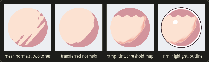
The first two images of the figure show the same effect on a whole sphere covered with small bumps: with mesh normals the shadow border shatters; with 85% transferred normals it becomes one clean, drawable shape.
Guilty Gear Xrd was made this way (Junya C. Motomura, "GuiltyGearXrd's Art Style: The X Factor Between 2D and 3D", GDC 2015): normals were edited on every major feature, faces most of all.
Thresholds, ramps and tints
The second tool is control over where the border falls.
The same talk stored a threshold offset in a vertex color channel: adding it to makes an area easier or harder to shade, and a value of 0 kept an area always in shadow.
A texture can do the same per pixel, a threshold map (しきい値マップ); in the third image of the figure, a wavy band painted into it makes the shadow of a fringe of hair that the geometry doesn't cast.
Some games at the time of writing go further and bake, for the face, a texture of the light angles at which each texel becomes shadowed, so the nose and cheek shadows follow hand-drawn shapes as the light turns.
The step itself is usually softened a little, with a smoothstep (a smooth 0-to-1 ramp, for clamped to ), and the shadow color is not a darker copy but the base color times a shadow tint, often shifted toward red or purple:
Worked example.
Threshold , half width , base color (skin) and shadow tint , so the shadow color is , darker and redder.
At with no offset: , , and the color is , almost lit.
With a threshold-map offset the same point has , so : shadow.
A ramp texture (section 16.9) can add a thin, saturated band right at the border, which imitates the warm edge painters put where light turns into shadow on skin; that's the reddish line in the third image.
Rim light and highlights
A rim light (リムライト) is a bright edge along the silhouette that separates the character from a dark background.
A cheap version uses the facing ratio , which falls to 0 at the silhouette:
The factor keeps it on the shadow side, where it reads best.
Example: gives , full rim; gives 0.65, halfway, ; gives 0.5, no rim.
Highlights are hard-edged shapes too: a step on instead of a Phong lobe, or a painted highlight texture for hair.
// Anime-style shading: soft two-tone step with a threshold offset, a shadow tint and a rim light.
float3 animeShade(float3 n, float3 l, float3 v, float3 baseColor, float3 shadowTint,
                  float thresholdOffset, float3 rimColor) {
  n = normalize(n);
  float nl = dot(n, normalize(l)) + thresholdOffset;  // offset from a vertex color or threshold map
  float lit = smoothstep(0.05, 0.15, nl);             // threshold 0.1, soft half width 0.05
  float3 color = lerp(baseColor * shadowTint, baseColor, lit);
  float rim = smoothstep(0.6, 0.7, 1.0 - saturate(dot(n, normalize(v)))) * (1.0 - lit);
  return color + rim * rimColor;                      // rim light on the shadow side only
}
// Anime-style shading: soft two-tone step with a threshold offset, a shadow tint and a rim light.
vec3 animeShade(vec3 n, vec3 l, vec3 v, vec3 baseColor, vec3 shadowTint,
float thresholdOffset, vec3 rimColor) {
n = normalize(n);
float nl = dot(n, normalize(l)) + thresholdOffset; // offset from a vertex color or threshold map
float lit = smoothstep(0.05, 0.15, nl); // threshold 0.1, soft half width 0.05
vec3 color = mix(baseColor * shadowTint, baseColor, lit);
float rim = smoothstep(0.6, 0.7, 1.0 - clamp(dot(n, normalize(v)), 0.0, 1.0)) * (1.0 - lit);
return color + rim * rimColor; // rim light on the shadow side only
}// Anime-style shading: soft two-tone step with a threshold offset, a shadow tint and a rim light.
float3 animeShade(float3 n, float3 l, float3 v, float3 baseColor, float3 shadowTint,
float thresholdOffset, float3 rimColor) {
n = normalize(n);
float nl = dot(n, normalize(l)) + thresholdOffset; // offset from a vertex color or threshold map
float lit = smoothstep(0.05, 0.15, nl); // threshold 0.1, soft half width 0.05
float3 color = lerp(baseColor * shadowTint, baseColor, lit);
float rim = smoothstep(0.6, 0.7, 1.0 - saturate(dot(n, normalize(v)))) * (1.0 - lit);
return color + rim * rimColor; // rim light on the shadow side only
}Beyond shading, such productions use the inverted hull of section 16.10 with per-vertex widths, draw inner lines into textures, often give each character its own light, and animate with held poses (Guilty Gear Xrd treated every frame as a key frame).
28.12 Line rendering in depth
Smooth silhouettes on meshes
The mesh silhouette test of section 16.10 uses face normals, so on a finely tessellated curved surface it produces a zigzag of mesh edges.
Aaron Hertzmann and Denis Zorin ("Illustrating Smooth Surfaces", SIGGRAPH 2000) treated the mesh as an approximation of a smooth surface instead.
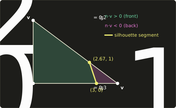
At each vertex compute with the interpolated vertex normal , the vertex position and the camera position .
Interpolate linearly over each triangle: the silhouette is its zero set, a straight segment through the triangles where changes sign.
Worked example.
A triangle has vertices , , (in its own plane) with , and .
On edge the sign changes at , the point .
On edge it changes at from : .
Edge has no sign change.
The silhouette crosses this triangle as the segment from to , and neighboring triangles continue it, because they share the crossing points on shared edges.
Suggestive contours
Contours alone often look too sparse: an artist adds lines along the side of a nose or under the eyes.
Doug DeCarlo, Adam Finkelstein, Szymon Rusinkiewicz and Anthony Santella ("Suggestive Contours for Conveying Shape", SIGGRAPH 2003) noticed that many such lines are contours from nearby viewpoints.
Let be the view vector projected onto the tangent plane.
Suggestive contours (示唆的輪郭, サジェスティブコンター) are the points where has a local minimum in the direction without reaching 0; equivalently, where the radial curvature (the normal curvature in the direction ) is zero and increasing toward .
If the surface turned a little more, that minimum would drop to 0 and become a real contour.
Example.
Along across a shallow dent, takes the values 0.62, 0.48, 0.41, 0.45, 0.58.
The minimum 0.41 is positive, so there's no contour, but it is a suggestive-contour point.
The paper filters weak ones with thresholds: the angle between and must exceed (they used 20° to 30°; here , so it passes), and the derivative of must exceed a small value, which removes noise on nearly flat regions.
Visibility, chaining and stylization
Lines extracted from the mesh (silhouettes, the creases of section 16.10, suggestive contours) are 3D curves; the renderer still has to decide which parts are visible, usually by testing points along each line against the depth buffer (with a small offset so a line isn't hidden by its own surface) or against an ID buffer.
Line stylization (線のスタイル化) then chains the visible segments into long strokes, parameterizes each by arc length, and renders it as a screen-space strip of triangles with a brush texture, tapered ends and a width that varies with depth, curvature or lighting (Blender's Freestyle is an example of such an engine).
Temporal coherence
A still image is easy; an animation is not.
From frame to frame, silhouette curves grow, shrink, split and merge, and a brush texture parameterized afresh each frame slides along the line or jumps.
Robert Kalnins and colleagues ("Coherent Stylized Silhouettes", SIGGRAPH 2003) carry the parameterization over: they render the previous frame's strokes into an ID image, look up which old stroke and parameter each new sample lands on, and fit a new parameterization that stays close to the old one.
Image-space lines (section 16.10) instead flicker on thin, distant features, which lines at least a pixel wide and temporal anti-aliasing reduce.
Temporal coherence (時間的一貫性) is what separates an NPR technique for still illustrations from one for games and film.
28.13 Real-time hatching with tonal art maps
Chapter 16 drew hatching in screen space, where strokes stick to the screen and the object slides behind them (the shower-door effect).
Attaching strokes to the surface with a texture solves that, but the tone changes continuously while a texture has a fixed stroke density, and a distant, minified texture shows its strokes smaller and denser than a pen would draw.
Emil Praun, Hugues Hoppe, Matthew Webb and Adam Finkelstein ("Real-Time Hatching", SIGGRAPH 2001) solved both with a tonal art map (トーナルアートマップ, TAM): a grid of hatching images, tones from light to dark in one direction and mipmap levels in the other.
The key is nesting (入れ子) in both directions:
- every stroke of a lighter tone appears in all darker tones, and
- every stroke of a coarser mip level appears in all finer levels.
Coarser levels contain fewer strokes, drawn with the same pixel width, so the stroke density on screen stays roughly constant at every distance.
Blending two nested images never makes strokes appear or vanish abruptly: it only fades in the extra strokes of the darker one.
They used 6 tones, packed into the red, green and blue channels of two textures, with blending weights computed per vertex; today the weights are computed per pixel.
Worked example.
Say the six tones have ink coverages 15%, 30%, 45%, 60%, 75% and 90%.
A pixel needs darkness , between tone 3 (0.45) and tone 4 (0.60).
The weights are and , and the average coverage is .
Because of nesting, the result shows all strokes of tone 3 at full strength plus the extra strokes of tone 4 at 46.7%.
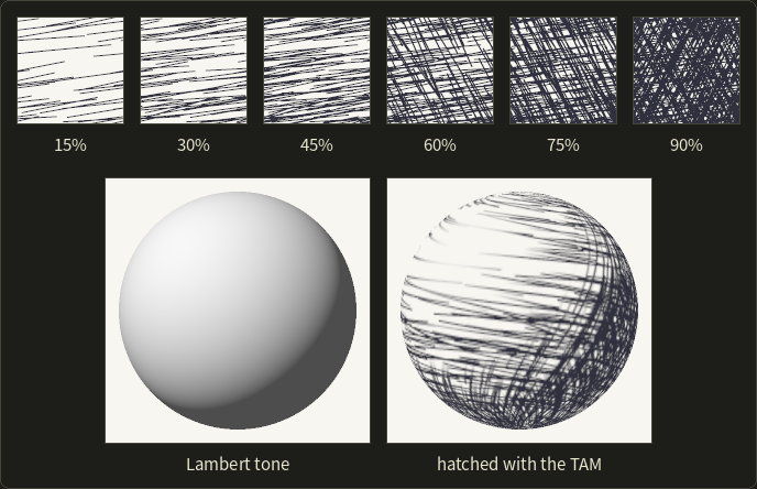
I built this TAM by adding random strokes to a tiling texture until each tone reached its coverage; the sphere uses longitude and latitude as texture coordinates, so the strokes follow the surface.
28.14 Painterly and watercolor rendering
Section 16.12 introduced stroke-based painterly rendering and Curtis et al.'s watercolor simulation (SIGGRAPH 1997).
Curtis's method simulates water and pigment physically, in layers, and composites the glazes with the Kubelka–Munk model; it reproduces dark edges, backruns and granulation, but slowly.
Real-time methods fake the look in image space.
Adrien Bousseau, Matt Kaplan, Joëlle Thollot and François Sillion ("Interactive Watercolor Rendering with Temporal Coherence and Abstraction", NPAR 2006) first simplify the image (removing small detail, as a painter would), then modulate every color with a pigment density read from textures: paper grain, low-frequency "turbulence" for uneven washes, and fine noise for pigment dispersion.
The color modification is
where is the texture value and a global strength; darkens (more pigment), lightens.
Example: for and , ; for , .
White () never changes, because the term is 0: unpainted paper stays paper.
The absolute effect is largest at mid tones, where peaks at 0.25.
Edge darkening (エッジの暗化), the dark rim where pigment collects at the border of a wash, is added from the image gradient, and wobbling distorts the image slightly along the gradient of the paper texture so edges look hand-painted.
For animation, the textures must move with the scene and not with the screen (the shower-door problem again); Barbara Meier ("Painterly Rendering for Animation", SIGGRAPH 1996) attached brush strokes to particles on the 3D surfaces, which became the standard answer for stroke-based styles.
28.15 Stylization with image filters
The Kuwahara filter, worked
Chapter 16 described the Kuwahara filter: look at four overlapping square regions around a pixel and output the mean of the one with the smallest variance.
Here's a 5 × 5 neighborhood across a vertical edge (dark on the left, bright on the right), with a noisy center pixel of 30:
| col 0 | col 1 | col 2 | col 3 | col 4 | |
|---|---|---|---|---|---|
| row 0 | 10 | 12 | 11 | 80 | 82 |
| row 1 | 11 | 10 | 13 | 81 | 79 |
| row 2 | 12 | 11 | 30 | 78 | 80 |
| row 3 | 10 | 13 | 11 | 82 | 81 |
| row 4 | 14 | 12 | 10 | 79 | 80 |
The four 3 × 3 regions share the center pixel:
| Region | rows, columns | mean | variance |
|---|---|---|---|
| top left | 0–2, 0–2 | 13.33 | 35.56 |
| top right | 0–2, 2–4 | 59.33 | 879.56 |
| bottom left | 2–4, 0–2 | 13.67 | 34.89 |
| bottom right | 2–4, 2–4 | 59.00 | 911.33 |
The bottom-left region varies least, so the output is 13.67: the noise is gone and the pixel stays on the dark side of the edge.
A 3 × 3 mean filter would give 36.6, smeared across the edge.
Variants
The classic filter has flaws: the square regions produce blocky artifacts, and when two regions have almost equal variance (like 35.56 and 34.89 above), noise decides which one wins, so the output flickers.
- The generalized Kuwahara filter (一般化桑原フィルタ; Giuseppe Papari, Nicolai Petkov and Patrizio Campisi, IEEE Transactions on Image Processing, 2007) uses a circular window divided into (typically 8) sectors with smooth Gaussian weights, and blends the sector means with weights that fall steeply with the standard deviation, for example .
- The anisotropic Kuwahara filter (異方性桑原フィルタ; Jan Eric Kyprianidis, Henry Kang and Jürgen Döllner, Pacific Graphics 2009) stretches the circle into an ellipse aligned with the local edge direction (from the structure tensor, a smoothed matrix of products of image derivatives); the result looks like brush strokes following the shapes.
Example: apply the blended weighting to the four regions above with .
The standard deviations are 5.963, 29.66, 5.907 and 30.19; with the normalized weights are 0.481, 0.0000013, 0.519 and 0.0000011.
The output is : the two dark regions are averaged smoothly instead of one winning outright, and the bright regions count for practically nothing.
With the bright regions would still get about 2% each and pull the result up to 15.2: a larger means sharper edges.
DoG and XDoG
The difference of Gaussians (DoG, ガウス差分) subtracts two blurs of the image, ; it approximates the Laplacian of Gaussian of section 15.5, , and is the usual choice since Marr and Hildreth.
Holger Winnemöller and colleagues used thresholded DoG lines with bilateral filtering and color quantization to turn video into cartoons in real time ("Real-Time Video Abstraction", SIGGRAPH 2006), the cartoon-like abstraction mentioned in section 16.12.
The XDoG (Holger Winnemöller, Jan Eric Kyprianidis and Sven Olsen, "XDoG: An eXtended Difference-of-Gaussians Compendium Including Advanced Image Stylization", Computers & Graphics, 2012) makes it a stylization tool in two steps.
First, a sharpened image:
which is unsharp masking (chapter 15) with a strong edge boost (around 20).
Second, a soft threshold:
sets which tones turn dark and how sharp the transition is: a large gives black-and-white ink, a small one soft pencil or charcoal shading.
Worked example.
A 1D step from 0.2 to 0.8 at , with , , , and .
The blurred step is , with the cumulative normal distribution:
| −6 | 0.2000 | 0.2001 | 0.199 | 0.80 |
| −4 | 0.2000 | 0.2037 | 0.126 | 0.54 |
| −2 | 0.2137 | 0.2634 | −0.781 | 0.00 |
| −1 | 0.2952 | 0.3596 | −0.993 | 0.00 |
| 0 | 0.5 | 0.5 | 0.5 | 1 |
| 1 | 0.7048 | 0.6404 | 1.993 | 1 |
| 2 | 0.7863 | 0.7366 | 1.781 | 1 |
Far from the edge, equals the original value: the dark flat area (0.2) becomes a light gray tone of 0.80, the bright area white.
Next to the edge, on the dark side, overshoots far below 0 and the threshold makes a black line a few pixels wide.
So XDoG gives lines and tone together, from one formula.
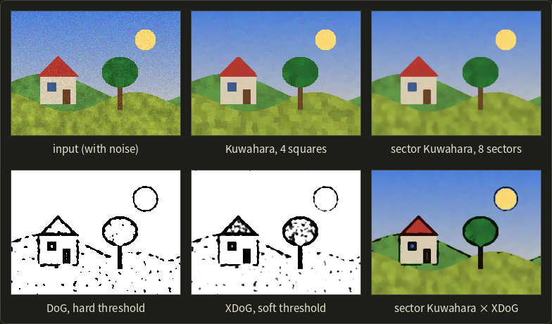
The classic Kuwahara result is blocky in the grass; the 8-sector version is rounder.
DoG and XDoG ran on the luminance after a light blur (σ = 1); XDoG fills the dark window, door and tree crown where DoG only outlines them, and the last image multiplies the Kuwahara colors by XDoG lines: a cheap cartoon filter.
Henry Kang, Seungyong Lee and Charles Chui ("Coherent Line Drawing", NPAR 2007) smooth the DoG along the local edge direction (flow-based DoG), which turns broken dashes into long coherent lines.
28.16 Style transfer and learned stylization
Section 16.12 introduced neural style transfer (Gatys, Ecker and Bethge, 2015): find an image whose deep features match a content image and whose feature statistics match a style image.
The statistics are Gram matrices (グラム行列): if a network layer has channels at positions, stored as a matrix , then
measures how strongly channels and respond together, regardless of where.
Example: two channels at three positions, , give (, , ).
Shuffling the three positions doesn't change : it keeps textures and brushwork but forgets layout, which is exactly what "style" should mean here.
Gatys's method optimizes each image from scratch, which takes minutes.
Justin Johnson, Alexandre Alahi and Li Fei-Fei (ECCV 2016) trained a feed-forward network per style with the same losses, fast enough for real time.
Xun Huang and Serge Belongie (ICCV 2017) allowed any style in one pass with adaptive instance normalization (AdaIN), which gives each content feature channel the mean and standard deviation of the style's channel: .
For video, stylization must also be temporally stable: methods add a loss that compares each frame with the previous one warped by optical flow (chapter 27).
At the time of writing, diffusion-based image generators (chapter 29) can also restyle images and video from a text prompt, and imitating a living artist's style raises the questions of section 18.7.
Games still mostly build their looks from hand-designed shaders like those of sections 28.11 to 28.15, for control, stability and cost.
Exam points
These tie back to non-photorealistic rendering (chapter 16):
- Anime-style shading controls the toon step's inputs: edited or transferred normals, threshold offsets (vertex colors, threshold maps), ramps and shadow tints; rim light from .
- Contours of a smooth surface: zero set of (interpolated within triangles); suggestive contours: positive local minima of in the projected view direction (radial curvature 0), i.e. contours of nearby views.
- Temporal coherence is essential for animation: strokes attached to the surface (no shower door), parameterizations carried across frames.
- Tonal art maps: hatching textures for several tones and mip levels, nested so blending is smooth and screen density stays constant.
- Kuwahara: the mean of the least varied subregion keeps edges; DoG ≈ LoG; XDoG = sharpened image + soft threshold, giving lines and tones.
- Style transfer matches Gram-matrix statistics of deep features.
28.17 Summary
- A participating medium absorbs, scatters and emits light (, , , albedo, phase function); transmittance is , and optical depths add.
- The volume rendering integral adds emission and in-scattering along a ray, dimmed by the transmittance to the eye; the emission–absorption model of DVR becomes front-to-back compositing with , with opacity correction when the step changes.
- Henyey–Greenstein phase functions have one parameter, the mean cosine . Ray marching with single scattering integrates each step analytically, with a shadow march toward the light; multiple scattering is approximated by octaves or path traced with delta and ratio tracking.
- Skies use Rayleigh, Mie and ozone layers with small tables; games light fog in froxels and ray march clouds with temporal reuse; visualization uses 3D textures, empty-space skipping, early termination and pre-integration.
- Anime-style shading controls normals, thresholds, ramps, tints and rims; lines add smooth silhouettes, suggestive contours, stylized strokes and temporal coherence; tonal art maps give coherent hatching; watercolor modulates pigment density; Kuwahara variants and XDoG stylize images; style transfer matches Gram matrices.
28.18 Key terms
| English | 日本語 |
|---|---|
| participating medium | 関与媒質 |
| absorption, out-scattering, in-scattering, emission | 吸収、外向き散乱、内向き散乱、放射(発光) |
| absorption coefficient | 吸収係数 |
| scattering coefficient | 散乱係数 |
| extinction coefficient | 消散係数(減衰係数) |
| single-scattering albedo | 散乱アルベド |
| mean free path | 平均自由行程 |
| homogeneous / heterogeneous medium | 一様な媒質/非一様な媒質 |
| transmittance | 透過率 |
| optical depth | 光学的厚さ |
| Beer–Lambert law | ランベルト・ベールの法則 |
| radiative transfer equation (RTE) | 放射伝達方程式 |
| volume rendering integral | ボリュームレンダリング積分 |
| emission–absorption model | 放射・吸収モデル |
| opacity correction | 不透明度の補正 |
| phase function | 位相関数 |
| scattering angle | 散乱角 |
| isotropic scattering | 等方散乱 |
| Henyey–Greenstein phase function | ヘニエイ・グリーンスタイン位相関数 |
| asymmetry parameter | 非対称パラメータ |
| ray marching | レイマーチング |
| single scattering, multiple scattering | 単一散乱、多重散乱 |
| delta tracking (Woodcock tracking) | デルタトラッキング(ウッドコック・トラッキング) |
| majorant | 優関数(メジャラント) |
| null collision | ヌル衝突 |
| ratio tracking | 比率トラッキング |
| aerial perspective | 空気遠近法 |
| froxel | フロクセル |
| 3D texture | 3次元テクスチャ |
| empty-space skipping | 空領域スキップ |
| pre-integrated transfer function | 事前積分伝達関数 |
| edited normals, normal transfer | 法線編集、法線転写 |
| threshold map | しきい値マップ |
| rim light | リムライト |
| suggestive contour | 示唆的輪郭(サジェスティブコンター) |
| line stylization | 線のスタイル化 |
| temporal coherence | 時間的一貫性 |
| tonal art map (TAM) | トーナルアートマップ(TAM) |
| pigment density | 顔料密度 |
| edge darkening | エッジの暗化 |
| generalized Kuwahara filter | 一般化桑原フィルタ |
| anisotropic Kuwahara filter | 異方性桑原フィルタ |
| difference of Gaussians (DoG) | ガウス差分(DoG) |
| XDoG | XDoG |
| Gram matrix | グラム行列 |
| adaptive instance normalization (AdaIN) | 適応的インスタンス正規化(AdaIN) |
28.19 Challenges
- ★ A fog has and per meter. Compute , the albedo, the mean free path and the transmittance over 5, 10 and 20 m. Light then crosses 4 m of this fog and 6 m of air with per meter: what is the total transmittance?
- ★ Evaluate the HG phase function with at 0°, 90° and 180°, and check that the forward-to-backward ratio is . Which value of gives a ratio of 27?
- ★★ With the emission–absorption model, composite four segments of length with and in front of a background of 1. Then a transfer function designed for gives : what opacity must a renderer use with steps of 0.1, and what with steps of 0.5?
- ★★ Delta tracking by hand: , for and for , ray length 4. With , list the tentative collisions and the ratio-tracking estimate of the transmittance. Compare with the exact value and explain the difference.
- ★★ A froxel grid has m, m and exponential slices. Compute the depth ratio between slices, the thickness of the first and the last slice, and which slice contains the depth 10 m. How much memory does a 240 × 135 × 128 volume of four 16-bit floats need?
- ★★ Apply the classic Kuwahara filter (four 3 × 3 regions) to the center of the 5 × 5 patch with rows (50, 52, 49, 51, 50), (48, 51, 50, 120, 122), (50, 49, 90, 121, 119), (52, 50, 118, 120, 121), (49, 51, 119, 122, 120). Then blend the four region means with and compare.
- ★★★ Why do the single-scattering clouds in the figure have dark gray interiors? What does the octave approximation of section 28.6 fake, and when might a renderer prefer delta tracking to ray marching despite the noise?
Multiple choice
Q1 ★ Which of the following statements about participating media is correct?
| A | The extinction coefficient is the absorption coefficient minus the scattering coefficient. |
| B | The transmittance through two consecutive layers is the product of their transmittances, because their optical depths add. |
| C | Out-scattering adds light to a ray from other directions, which makes fog glow around lamps. |
| D | A medium with a single-scattering albedo of 0 scatters light but never absorbs it. |
| E | Doubling the distance through a homogeneous medium halves the transmittance. |
Q2 ★★ Which of the following statements about the Henyey–Greenstein phase function with is correct?
| A | Because the function is normalized, its values at 0° and 180° are equal. |
| B | The parameter means that exactly half of the scattered light goes into the forward hemisphere. |
| C | Its value at 0° is . |
| D | A negative would make the scattering more strongly forward than . |
| E | Its value at 0° is 27 times its value at 180°. |
Q3 ★ Which of the following statements about NPR techniques is correct?
| A | In a tonal art map, each darker tone uses a new, unrelated set of strokes so that the hatching does not look repetitive. |
| B | Suggestive contours are the points of a surface where . |
| C | The soft threshold of XDoG maps every value below to exactly 0. |
| D | The Kuwahara filter outputs the mean of the subregion with the smallest variance, which smooths flat areas while keeping edges sharp. |
| E | Transferring normals from a proxy sphere to a face makes the toon shadow borders follow small geometric details more closely. |
28.20 Practical assignment
A cloud ray, a phase function and an anime sphere, by hand.
You need graph paper, a ruler, a protractor, colored pencils and a calculator.
Part A: one ray through a cloud.
A camera ray crosses five 1 m cells with per meter and albedo 0.9 (so ).
The sun's transmittance to the cells, , is 1, 0.8, 0.5, 0.3 and 0.6; the sun's intensity is ; the phase function is HG with at a scattering angle of 60°; behind the cloud is sky with .
- Phase. Compute at 60° for .
- Table. For each cell write the transmittance at its start, the source , the factor (use 1 for the empty cell) and the contribution times that factor. Add up and the background term.
- Compare. Repeat with the naive contribution m. Which cells cause most of the difference, and why?
Part B: the HG phase function on paper.
For , compute at .
- Polar plot. With the incoming light along the horizontal axis, mark each value as a distance from the center in its direction (2 cm per unit), mirror the points below the axis and join them into a closed curve. Draw the unit circle (isotropic scattering) for comparison.
- Normalization. Estimate with Simpson's rule on the same seven angles (step , weights 1, 4, 2, 4, 2, 4, 1 times ).
Part C: an anime-style sphere.
Draw a circle of radius cm, a sphere seen from the front (), lit from .
On the horizontal diameter the normal at is .
- Values. For , compute , the lit factor and the rim .
- Color. Use the skin colors of section 28.11 (base , shadow ) and color the disk: lit side, the narrow soft border, shadow, and a white rim where .
- Threshold map. Now add an offset in the band (a hair shadow) and redraw that band. Where does the border move?
How to check yourself:
- Part A: ; the transmittance after the cloud is , so the background adds 0.0371; the energy-conserving total is about 0.448 (0.485 with the background), the naive one about 0.646 (0.683). The dense third cell is where the naive sum overshoots most.
- Part B: the values are 6, 3.152, 1.155, 0.537, 0.324, 0.244 and 0.222 (the ratio of the first to the last is 27); Simpson's rule gives about 1.004, close to 1.
- Part C: is largest (1) at ; the border () crosses the diameter at , and the soft band runs from about to ; the rim appears only on the shadow side, beyond (), and reaches full strength beyond . With the offset, the shaded band reaches far into the lit side, since there must exceed 0.6 to be lit.
コメント(0)
まだコメントはありません。
ログインするとコメント出来ます。