8. Curves and Surfaces
A car body, the hull of a ship, the letter "S" on this page, the path a camera flies along in a cutscene: none of them is made of straight lines or flat triangles, at least not in the file the designer saved.
They are free-form curves and surfaces (自由曲線・自由曲面), described by a handful of points and a formula that fills in everything in between.
In this chapter I'll build those formulas one by one: Hermite curves, Bézier curves, B-splines and NURBS, the interpolating splines that pass through every point, and finally the surfaces made from them.
Why does this matter?
CAD systems, font formats, vector drawing programs, animation curves and film modeling tools are all built on exactly these few families of curves, and when you know how they work you know why a pen tool has "handles", why a circle in a CAD file needs weights, and why a moved point changes the whole curve in one program and only a small part in another.
For the exam, this chapter covers the syllabus item 曲線・曲面 (curves and surfaces) of area 3, モデリング (modeling).
Chapter 7 is about how whole solids are represented; the faces of those solids in a CAD model are usually exactly the surfaces of this chapter.
Polygon meshes and subdivision surfaces come in chapter 9.
You'll need vectors and linear combinations (Linear Algebra chapter 2), the cross product (chapter 5), matrix–vector products (chapter 6) and homogeneous coordinates (chapter 9), plus the affine and projective transforms of chapter 4 and the perspective division of chapter 5.
There is a little calculus too, but only one kind: the derivative of a polynomial, .
That's all we need for tangents.
8.1 Three ways to describe a curve
Here are three ways to write down a curve in the plane:
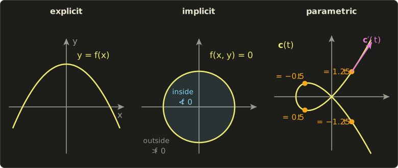
- Explicit form (陽関数表現): . For every there is exactly one . Example: .
- Implicit form (陰関数表現): . The curve is the set of points where a function is zero. Example: the unit circle . The sign of tells you on which side you are: inside, outside.
- Parametric form (パラメトリック表現, also 媒介変数表現): . A parameter runs through an interval, and each value gives a point. Example: the unit circle again, for .
Each one has its strengths:
| Form | Easy | Hard |
|---|---|---|
| explicit | evaluating, plotting a graph | vertical tangents, closed curves, more than one per (a circle needs two functions) |
| implicit | inside/outside test, closed shapes | generating points along the curve (you have to solve an equation) |
| parametric | generating points in order, any shape in 2D or 3D, self-intersections | inside/outside test |
The curve on the right of the picture is .
It crosses itself at the origin (for and ), so no explicit could describe it, yet the parametric form handles it without trouble.
Computer graphics uses the parametric form for almost all modeling curves and surfaces, for three reasons.
First, drawing is easy: step from start to end and connect the points.
Second, it works the same in 3D: just add .
Third, as we'll see, the curves of this chapter are controlled by points, and transforming the control points transforms the whole curve.
Implicit surfaces have their own uses (metaballs, signed distance fields), and chapter 9 covers them.
The tangent vector
Differentiate each coordinate of a parametric curve and you get the tangent vector (接線ベクトル) .
It points in the direction the point is moving, and its length is the speed at which it moves as increases.
For the self-crossing curve, , so at :
That's the pink arrow in the picture (drawn shorter so it fits).
For the circle , , which always has length 1 and is always perpendicular to the radius, as a tangent to a circle should be.
Remember the difference between direction and speed: the shape of a curve only depends on the direction of the tangent, while the length depends on how fast the parameter runs.
The same circle traced with has tangents twice as long.
That difference is the whole story of the next section.
Why polynomials, and why cubic
The curves in this chapter use polynomials in for each coordinate, because polynomials are cheap to evaluate, easy to differentiate and easy to reason about.
A single polynomial of high degree is hard to control, though, so long curves are built from several short pieces: a piecewise polynomial curve, which is what the word spline (スプライン) means.
(The name comes from the thin flexible strips of wood that shipbuilders and draftsmen bent through fixed points to draw smooth hull lines.)
Most pieces are cubic (3次), degree 3:
with four coefficient vectors .
Degree 3 is the smallest degree that can do everything we need: a cubic can have an inflection point (an S shape) in the plane, it can twist out of a plane in 3D (a quadratic always lies in one plane), and its four coefficients are exactly enough to fix both endpoints and both end tangents, so neighboring pieces can be joined smoothly.
The rest of the chapter is mostly about how to choose those four vectors from points a designer can move around.
8.2 Continuity
When two pieces meet, how smooth is the joint?
Let the first piece end where the second piece starts, both with .
There are two ways to measure the smoothness.
Parametric continuity (パラメトリック連続性) compares derivatives as vectors:
- (C0連続): the pieces meet, . There may be a corner.
- (C1連続): also , the same tangent vector, direction and length.
- (C2連続): also , the same second derivative.
Geometric continuity (幾何学的連続性) only asks about the shape:
- : the same as , the pieces meet.
- : the tangent directions agree, for some . The lengths may differ. No visible corner.
- : also the curvature (曲率) agrees, so the curve bends equally sharply on both sides of the joint.
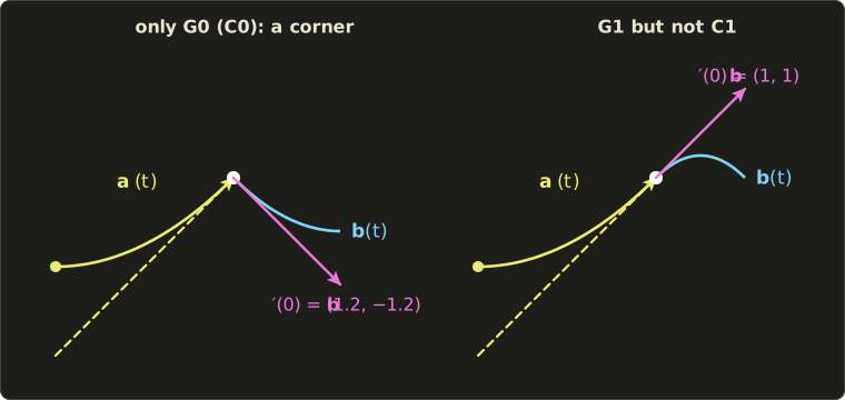
A worked example: G1 but not C1
Take and .
- Do they meet? and . Yes, so and .
- Tangents. , so . , so .
- Compare. : the same direction with , so the joint is . But , so it's not .
On the screen you see a perfectly smooth joint (right half of the picture).
But a point moving along the curve at constant steps of suddenly slows down to half speed at , because the second piece covers less distance per unit of .
If this curve were a camera path, you'd feel that jolt.
And notice that we can fix it without changing the shape at all: running twice as fast, for , gives , and the joint becomes .
That's the difference in one sentence: G-continuity is about the shape, C-continuity is about the shape and the parameterization.
The left half of the picture shows a joint that is only : the second piece leaves in the direction , which is not a positive multiple of , so there is a corner.
Which continuity for which job
- is enough for a shape to look smooth in a silhouette.
- matters for shiny surfaces: reflections and highlights run across a joint with a visible kink in their curvature. Car designers ask for (or more) on visible body panels.
- and matter when the parameter is time: a path has continuous velocity, a path also continuous acceleration, which is what you want for camera moves and animation curves (chapter 13).
A trap worth knowing for the exam: usually implies , but not always.
If both tangent vectors are zero at the joint, they are equal (so ), yet they have no direction, and the curve can have a sharp corner there.
8.3 Hermite curves
The most direct way to pin down a cubic piece is to say where it starts and ends and in which direction it leaves and arrives.
A Hermite curve (エルミート曲線) is the cubic with
two endpoints and two tangent vectors.
Finding the coefficients
Put and into the four conditions:
The first two give and directly.
The last two are two equations in and , and solving them gives
Basis functions
Collect the terms that multiply each of the four inputs, and the curve becomes a weighted sum:
The four polynomials are the Hermite basis functions (エルミート基底関数).
This is the pattern of every curve in this chapter: fixed basis functions (基底関数) of , multiplied by the data a designer controls, and added up.
The basis functions decide the character of the curve type; the data decides the particular curve.
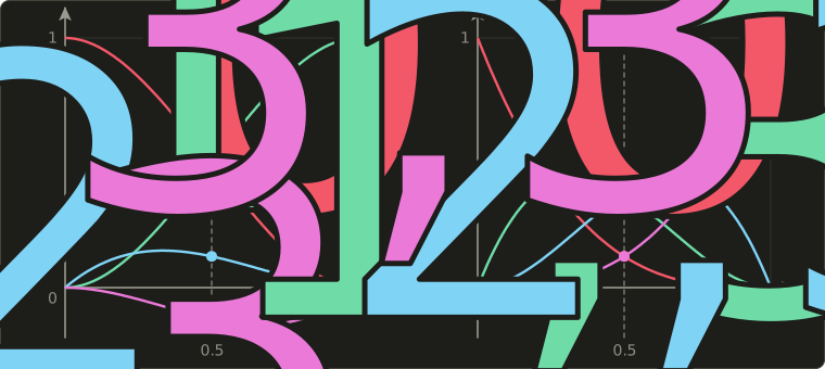
On the left you can read off why it works: at only is 1 (so the curve starts at ), at only is 1, and and are zero at both ends but have slope 1 at one end, which is how the tangents get in.
for every , so the point part is a proper weighted average.
Matrix form
The same thing as a product of a row of powers of , a fixed matrix, and a column of the data:
Read it as: the row times the matrix gives the four basis function values (the first column of the matrix holds the coefficients of , and so on), and those multiply the four data vectors.
The right-hand column is a "column of points", so you do the last step once for x and once for y (and z).
Every cubic curve type has such a basis matrix (基底行列); changing the matrix changes the curve type.
A worked example
Let , , and .
At : , , and (the dots in the picture). So
The coefficients check out too: and , so , and at that's .
Keep this point in mind; the next section reaches it from a completely different direction.
Where Hermite curves are used
Hermite form is natural whenever tangents are what you know: the keyframe curves of animation software, where each key has an "in" and an "out" tangent; motion paths; and joining pieces, because if neighboring pieces share the endpoint and the tangent vector, the joint is automatically .
Its weakness is that tangent vectors are awkward to edit by hand, which is exactly what the next curve fixes.
8.4 Bézier curves
A Bézier curve (ベジェ曲線) is controlled by a list of control points (制御点) .
The curve starts at the first one, ends at the last one, and is pulled towards the ones in between without (usually) touching them.
Joining the control points in order gives the control polygon (制御多角形), and the curve follows its general shape like a smoothed copy.
The curves were developed independently in the car industry around 1960: by Paul de Casteljau at Citroën (documented in 1959) and by Pierre Bézier at Renault, who published them and whose name stuck.
Today they are in every vector drawing program, in fonts (TrueType outlines use quadratic Bézier curves, PostScript and CFF outlines cubic ones), in SVG paths and in CSS cubic-bezier() easing curves.
Bernstein polynomials
The Bézier curve of degree with control points is
The weights are the Bernstein polynomials (バーンスタイン多項式, the Bernstein basis functions).
The fraction in front is the binomial coefficient you know from Pascal's triangle: 1, 3, 3, 1 for .
So a cubic Bézier curve is
Look at the right half of the basis picture.
All four weights are never negative, and they always add up to 1, because they are the terms of .
So every point of the curve is a weighted average of the control points: that one fact gives most of the properties below.
At the weights are .
With the control points , , , :
The same point as the Hermite example.
That's no coincidence, and we'll see why in a moment.
De Casteljau's algorithm
There's a beautiful way to compute the same point with nothing but linear interpolation (線型補間), , the point a fraction of the way from to .
De Casteljau's algorithm (ド・カステリョのアルゴリズム): interpolate each pair of neighbors in the control polygon, which gives one point fewer; repeat on the new points; when one point is left, that's .
Let's do it for our curve at , where every interpolation is just a midpoint:
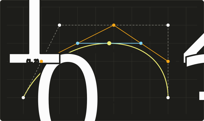
The first three lines are level 1, the next two level 2, and the last one level 3.
The last point, , matches the Bernstein computation exactly.
For a other than 0.5 you do the same thing with "go a fraction of the way" instead of "take the midpoint" (challenge 1 does ).
Why does it work?
Expand the levels: each step multiplies by or by , and after three levels arrives along different paths, each with the weight . That's exactly the Bernstein polynomial.
De Casteljau's algorithm only ever takes weighted averages of points, so it's numerically very stable, which is why it's the standard way to evaluate Bézier curves in software.
The construction gives two bonuses for free:
- The tangent. The last segment, from to , touches the curve at , and for a cubic. Here : at the curve is moving horizontally, at its highest point.
- Subdivision (分割). The points along the left edge of the triangle, = , are the control points of the left half of the curve, and the right edge, , of the right half. Each half is again a cubic Bézier curve, and its control polygon hugs the curve more closely than the original.
Subdivision is how renderers draw Bézier curves: split until each piece's control polygon is almost a straight line, then draw that line.
The same trick finds intersections of curves (split both until the pieces are tiny) and is the foundation of rendering fonts.
Derivatives and the end tangents
Differentiating the Bernstein form gives another Bézier curve, one degree lower, whose control points are the differences of the original ones:
At the ends only one term survives:
The curve leaves along the first leg of the control polygon and arrives at along the last leg.
For our cubic, and .
These are exactly the and of the Hermite example, which explains why both gave : they are the same curve.
Cubic Bézier and Hermite: the conversion
A cubic Bézier curve and a Hermite curve are two descriptions of the same set of cubics:
(The Hermite end point called in section 8.3 is the Bézier here.)
That's the secret of the "handles" in Illustrator, Inkscape or the pen tool of any drawing program: a handle is the inner control point, and dragging it sets the tangent at the anchor point: the tangent vector is three times the handle.
The cubic Bézier also has a basis matrix:
With the row times this matrix gives again.
Properties
These are the properties to know by heart:
- Endpoint interpolation (端点補間): the curve passes through and , and in general through no other control point.
- End tangents: the curve is tangent to the first and last legs of the control polygon there.
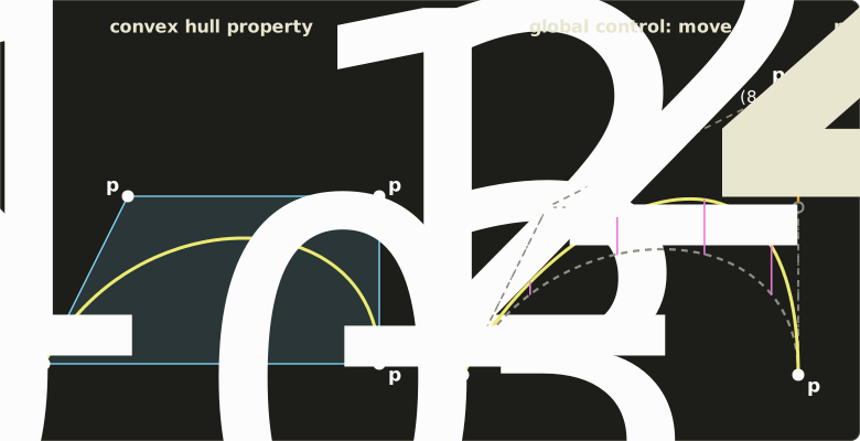
- Convex hull property (凸包性): the whole curve lies inside the convex hull (凸包) of its control points, the smallest convex region containing them (think of a rubber band stretched around the points). That follows from the weights being non-negative and adding up to 1. It's used for quick rejection: if the convex hulls of two curves don't overlap, the curves can't intersect, and if a hull is entirely off screen, so is the curve.
- Affine invariance (アフィン不変性): to apply an affine transform (chapter 4) to the curve, apply it to the control points and draw the curve of the new points; you get exactly the transformed curve. This works because an affine transform preserves weighted averages whose weights add up to 1.
- Variation diminishing property (変動減少性): in the plane, no straight line crosses the curve more often than it crosses the control polygon. The curve is never more wiggly than its polygon.
- Global control (大域的制御): every Bernstein polynomial is positive for all , so moving any one control point moves every point of the curve except the endpoints.
- The degree is tied to the number of points: control points always means degree .
A quick check of affine invariance with numbers: rotate by 90° and translate by , .
The control points become , and the Bernstein weights at give .
Transforming the old curve point directly gives .
Same point.
Careful, though: this is only true for affine transforms; a perspective projection of the control points does not give the projected curve.
We'll come back to that with NURBS.
Degree elevation
Sometimes you need a curve of higher degree with the same shape, for example to make a quadratic piece fit into a system that only handles cubics.
Degree elevation (次数上げ) turns control points into without changing the curve:
Example: the quadratic with becomes a cubic with and .
Check at : the quadratic gives , the cubic .
This is how a font converter turns TrueType's quadratic outlines into cubic ones without any loss.
Joining Bézier segments
Long shapes are chains of cubic segments.
Let the first segment have control points and the next one .
From the end tangent formula:
- : .
- : also , , lie on one straight line, with between the other two.
- : also equal legs, , which means (the mirror image of in ).
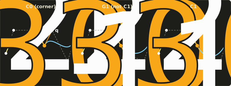
In the picture the first segment is , so its last leg is .
On the right, gives .
In the middle, is on the same line but only half as far, which gives but not , like the example of section 8.2.
On the left, is off the line, and you see a corner.
This is exactly the difference between a "smooth" anchor point (handles locked on a line) and a "corner" anchor point in a drawing program, and the "symmetric" option that also locks the handle lengths gives .
Getting across a joint by hand is much harder, and that's one reason for the next curve type.
8.5 B-spline curves
Bézier curves have two drawbacks for long, complicated shapes: every control point affects the whole curve, and more control points means higher degree.
The usual way around both is to chain cubic segments, but then the designer has to maintain the continuity conditions at every joint.
B-spline curves (Bスプライン曲線) do the chaining automatically: any number of control points, a fixed low degree, local control, and continuity built in for cubics.
Knots and the knot vector
A B-spline of degree (次数) is a piecewise polynomial of degree .
Its order (階数) is , the number of coefficients per piece; a cubic B-spline has degree 3 and order 4. (Watch out: some books number B-splines by order, some by degree.)
The pieces meet at parameter values called knots (ノット), listed in a non-decreasing knot vector (ノットベクトル) .
With control points and degree , the knot vector has entries.
The curve is again a weighted sum of control points:
and the weights , the B-spline basis functions (Bスプライン基底関数), are built from the knots by the Cox–de Boor recursion (コックス・ド・ブーアの漸化式):
with the rule that a fraction with denominator 0 counts as 0 (that happens when knots repeat).
Degree 0 is a box that is 1 on one knot span and 0 elsewhere.
Each step up blends two neighboring functions of the degree below with ramps that go from 0 to 1, so degree 1 gives tents, degree 2 smooth bumps over three spans, degree 3 bells over four spans.
Three kinds of knot vectors are worth naming:
- Uniform (一様): equally spaced knots, such as . All basis functions are shifted copies of each other. The curve generally doesn't start or end at a control point.
- Open uniform (開一様), also called clamped: the first and last knots are repeated times and the inner knots are equally spaced, such as for . Then the curve starts at and ends at , tangent to the first and last legs, like a Bézier curve.
- Non-uniform (非一様): any other spacing, including repeated inner knots. A knot repeated times lowers the continuity there from to , which lets a designer put a deliberate crease or corner into an otherwise smooth curve.
A worked example with Cox–de Boor
Degree , four control points (), so knots: the open uniform vector
The parameter runs from 0 to 2, with two pieces, and .
Let's evaluate at , which lies in the span .
Degree 0. Only the box of that span is on: , all other .
Degree 1. Only the functions that use can be nonzero, and :
(The first fraction of has the denominator , so it counts as 0.)
Degree 2. Now , and can be nonzero:
and .
Check: .
B-spline basis functions also add up to 1 everywhere, and they are never negative, so again every curve point is a weighted average.
With the control points , , , :
At the inner knot , the same recursion gives and the others 0, so , the midpoint of the middle leg.
(That's a general fact for quadratic B-splines with simple knots: the joints sit at midpoints of the control polygon's legs.)
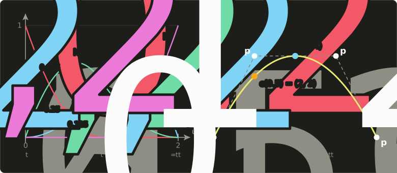
Notice that the curve starts at and ends at because the knot vector is clamped, but it doesn't touch or .
In practice, the evaluation is done with de Boor's algorithm, a generalization of de Casteljau's algorithm that interpolates control points with ratios taken from the knots, but Cox–de Boor is the definition and the version worth practicing on paper.
Local control
is zero outside the spans from to (its support, 台).
So control point only influences the part of the curve with , and conversely, each piece of the curve depends on only control points (four for a cubic).
This is local control (局所制御), the most important practical advantage of B-splines.
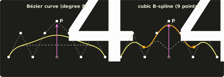
Both curves use the same nine control points, and in both I moved up by 3.
The Bézier curve (degree 8) changes everywhere, and it also follows its control polygon only very loosely.
The cubic B-spline uses the clamped knot vector ; lives on , so only the orange part between the two orange dots changed, and the yellow ends are exactly where they were (the dashed old curve is hidden under them).
A B-spline also has a stronger convex hull property: each piece lies inside the convex hull of its own control points, which hugs the curve much more tightly than the hull of all points.
The uniform cubic B-spline
With uniform knots, every cubic piece has the same formula.
The piece that uses the four control points is, with a local parameter :
At the weights are , at they are and at they are .
With :
The piece passes through none of its control points: a uniform B-spline approximates its control points.
Why is it ?
Differentiate the matrix form twice and evaluate at the ends.
The end of the piece that uses has
and the start of the next piece, which uses , has
Identical, all three, whatever the control points are.
So the continuity comes from the basis functions themselves, and the designer can move points freely without ever breaking it.
That's the deal: you give up passing through the control points and get automatic smoothness plus local control in exchange.
Relation to Bézier curves
Bézier curves are a special case of B-splines.
A degree-3 B-spline with four control points and the knot vector has exactly the Bernstein polynomials as its basis functions, so it is the cubic Bézier curve.
In the other direction, every B-spline can be cut into Bézier pieces by inserting knots until each inner knot is repeated times (knot insertion, ノット挿入), which is how many renderers and file converters handle them.
8.6 NURBS
Here's a problem that no curve so far can solve: draw an exact circle.
Polynomial curves can only approximate it (challenge 5 asks you why).
That's a real problem for CAD: a drilled hole, a cylinder or a fillet has to be exactly round.
The answer is NURBS (ナーブス), non-uniform rational B-splines (非一様有理Bスプライン): B-splines with arbitrary knots (non-uniform) whose points are divided by a weighted sum (rational, a ratio of polynomials).
Weights and the rational form
Give every control point a weight (重み) :
If all weights are equal, they cancel and we're back to an ordinary B-spline.
Increasing pulls the curve towards , decreasing it pushes the curve away.
The same formula reads much more simply in homogeneous coordinates (同次座標, Linear Algebra chapter 9).
Write each control point with its weight as a homogeneous point in 2D, or in 3D.
Then:
- Evaluate an ordinary polynomial B-spline (or Bézier curve) of the homogeneous points.
- Divide by the last coordinate.
That second step is exactly the perspective division of chapter 5.
So a NURBS curve is a polynomial curve in one dimension higher, projected back by the division by w.
A quarter circle, exactly
Take a quadratic Bézier curve (which is also a NURBS curve, with knots ) with control points
At , the quadratic Bernstein weights are .
Homogeneous control points: , , .
Step 1, the polynomial curve in homogeneous coordinates:
Step 2, divide by the last coordinate:
and : exactly on the unit circle, at 45°.
At the same steps give , and .
In fact for every (challenge 5).
Compare the ordinary, non-rational quadratic Bézier curve with the same three points (all weights 1): at it gives , at distance from the center, 6% too far out.
It's a parabola, not a circle.
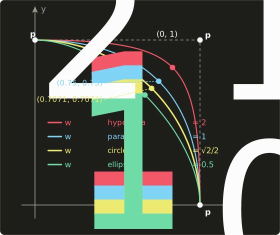
The picture shows the whole family.
With the end weights fixed at 1, the middle weight of a rational quadratic Bézier curve decides which conic section (円錐曲線) you get: gives an arc of an ellipse, a parabola, a hyperbola.
With this particular right-angled, equal-legged control triangle, the ellipse for is the circle.
A full circle is four such arcs: nine control points (the corners and edge midpoints of a square, the first repeated at the end), weights alternating , degree 2 and the knot vector .
Projective invariance
Because a NURBS curve is defined through homogeneous coordinates, it's projectively invariant (射影不変): apply a projective transform (even a perspective projection) to the homogeneous control points, and the curve of the new points is exactly the projected curve.
A plain Bézier or B-spline curve is only affine invariant, because projecting its control points changes their effective weights.
With NURBS, a perspective view of a circle is computed exactly by transforming nine points.
Why CAD uses NURBS
- One format for everything: lines, circles, ellipses, cylinders, cones, spheres and tori are represented exactly, and free-form shapes with the same machinery. A CAD kernel needs only one curve type and one surface type.
- Bézier curves and ordinary B-splines are special cases (all weights equal).
- Local control, the convex hull property (for positive weights) and well-understood algorithms (knot insertion, degree elevation, de Boor evaluation).
- Invariance under affine and projective transforms.
- It's the standard: the CAD exchange formats IGES and STEP store free-form geometry as NURBS, and modelers such as Rhino are built around them.
The price is more data per point (a weight, and a knot vector to manage) and the division, and that a NURBS surface needs to be tessellated into triangles before a GPU can draw it.
8.7 Interpolating splines
Interpolation versus approximation
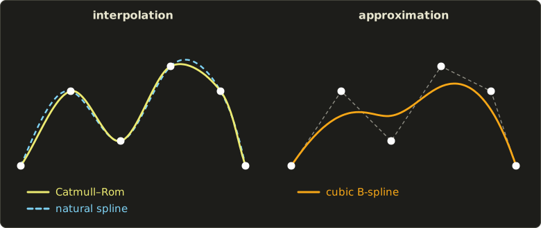
Bézier curves and B-splines approximate (近似) their control points: the curve is pulled towards them but generally doesn't pass through them.
That's ideal for designing shapes by eye, but sometimes you have points the curve must go through: measured data, keyframe values, the waypoints of a camera path.
A curve that passes through all given points is said to interpolate (補間) them.
Catmull–Rom splines
The Catmull–Rom spline (カトマル・ロム・スプライン, after Edwin Catmull and Raphael Rom) is the simplest interpolating spline.
For the segment between and , use a Hermite curve whose tangents are taken from the neighbors:
The tangent at each point is parallel to the line through its two neighbors.
Neighboring segments share the point and the tangent vector, so the curve is everywhere.
Each segment depends on four points, , so control is local.
The first and last segments are missing a neighbor; the usual fix is to invent one, by repeating the end point or mirroring its neighbor (the picture mirrors).
As a basis matrix:
Worked example. Points , middle segment from to :
With the Hermite weights at from section 8.3:
The matrix gives the same: its weights at are , and .
Note the negative weights: a Catmull–Rom spline has no convex hull property, and it can overshoot its points.
As a Bézier segment (section 8.4), the same piece has the inner control points and .
Catmull–Rom splines are everywhere in games and animation: camera paths through waypoints, the default "smooth" interpolation of keyframes (chapter 13), paths of moving platforms, smoothing a hand-drawn stroke.
Variants with an extra parameter (cardinal splines with a tension, Kochanek–Bartels splines with tension, continuity and bias) give the animator more control over how tight the curve is around each point.
Natural cubic splines
A Catmull–Rom spline is only .
If you want a curve that passes through every point, there's a classic answer: the natural cubic spline (自然3次スプライン).
With points there are cubic pieces, unknown coefficients, and these conditions:
- each piece passes through its two end points: equations;
- first and second derivatives agree at the inner points: equations;
- "natural" ends, second derivative zero at the first and last point: 2 equations.
That's equations for unknowns.
For equally spaced parameters, everything reduces to one small system for the second derivatives at the points:
(written for one coordinate ; do the same for x and z).
Tiny example: values at .
There's one unknown: , so .
On the first piece, with , the spline is , and at :
The catch is that this system couples all the points: moving one point changes every , and therefore the whole curve.
A natural spline has global control, which is why interactive tools prefer Catmull–Rom or B-splines.
The name refers to the draftsman's wooden spline from section 8.1: a thin strip bent through fixed points takes, approximately, the shape of the natural cubic spline, the one with the least bending, and with free ends it isn't bent at the ends.
| Curve | Passes through | Control | Continuity | Convex hull |
|---|---|---|---|---|
| Hermite | both end points, with the given tangents | (one piece) | joints when tangents are shared | no |
| Bézier | first and last control point | global | joints need care | yes |
| B-spline (uniform cubic) | none (clamped: first and last) | local | yes | |
| NURBS | like the B-spline | local | like the B-spline | yes, for positive weights |
| Catmull–Rom | every point | local | no | |
| natural cubic spline | every point | global | no |
8.8 Surfaces
Everything so far carries over to surfaces with one more parameter.
A parametric surface (パラメトリック曲面) is a map from a square of parameters to space:
Fix and let run, and you get a curve on the surface; the same with fixed.
These are the isoparametric curves (アイソパラメトリック曲線, 等パラメータ曲線), and the yellow wireframes in the pictures below are exactly those.
A piece of surface over one parameter square is called a patch (パッチ).
Tensor-product patches and the bicubic Bézier patch
The simplest recipe is the tensor product (テンソル積): take a curve type, and use its basis functions in both directions.
A bicubic Bézier patch (双3次ベジェ曲面) has a grid of control points , the control net (制御点網), 16 points in all:
Read it as "a curve of curves".
For a fixed , each row of the net is first evaluated as a Bézier curve in ; that gives four points, which are then the control points of a Bézier curve in .
The four corner points lie on the surface, the four boundary rows and columns are the Bézier curves of the boundary, and the four inner points pull the surface without touching it.
Everything about Bézier curves (convex hull, affine invariance, de Casteljau, subdivision) carries over.
Worked example. I'll keep the convention of this series with y up: the net lies over a grid in the ground plane, , with heights (rows going away from the viewer, towards −z):
| 0 | 0 | 0 | 0 | |
| 0 | 2 | 2 | 0 | |
| 0 | 4 | 4 | 0 | |
| 0 | 0 | 0 | 0 |
Evaluate at , where the Bernstein weights are in both directions.
- Rows in u. The x coordinate of every row is . The heights: row 0 gives 0, row 1 gives , row 2 gives , row 3 gives 0. So the four row points are , , , .
- Column in v. and .
The inner control points are up at heights 2 and 4, but the surface only reaches 1.6875 in the middle: the control net is a "cage" that the surface stays inside.
Normals from partial derivatives
For shading (chapter 10) we need the normal vector (法線ベクトル) of the surface.
The partial derivatives and (偏微分: differentiate in one parameter while holding the other fixed) are the tangent vectors of the two isoparametric curves through the point.
Both lie in the tangent plane, so their cross product (Linear Algebra chapter 5) is perpendicular to the surface:
For our patch we need the derivatives of the cubic Bernstein polynomials, (with ).
At , with , they are .
- : apply the derivative weights along each row, then the ordinary weights down the column. x: . Height: every row is symmetric (0, 2, 2, 0 and 0, 4, 4, 0), so . z doesn't change along a row. So .
- : apply the derivative weights to the four row points of step 1. x: 0, since every row point has . Height: . z: . So .
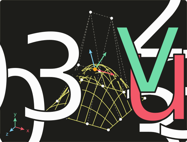
The normal points mostly up and a little towards +z, towards the viewer: the surface rises as you go away from the viewer (rows 1 and 2 have heights 2 and 4), so it faces slightly towards the near side, which makes sense.
The order matters: would point into the ground.
Which side is "outside" is a convention the modeling tool has to keep consistent.
B-spline and NURBS surfaces
Replace the Bernstein polynomials by B-spline basis functions, with one knot vector for and one for , and you get a B-spline surface; add weights, divide, and you get a NURBS surface (NURBS曲面):
All the curve properties carry over: local control, exact quadric surfaces (a sphere, a cylinder or a torus is an exact NURBS surface built from the circle arcs of section 8.6), projective invariance.
This is the surface type of CAD, and of the faces of B-rep solid models (chapter 7).
Coons patches
Sometimes the designer has the four boundary curves of a patch but no inner control points.
A Coons patch (クーンズ曲面, after Steven A. Coons) fills in the surface from its boundary.
With boundary curves , , , and corners , the bilinearly blended Coons patch is
The first line blends in : it stretches straight lines between the curves and .
The second line blends in , between and .
Adding both counts the corners twice, so the third line subtracts the bilinear interpolation of the four corners once.
The result matches all four boundary curves exactly.
Worked example. A square of side 2 on the ground: , , , and one arched side, , which rises to a height of 1 in its middle.
At : the blend in v is ; the blend in u is ; the corners blend to .
Halfway between the flat side (height 0) and the top of the arch (height 1), as you'd expect.
Coons patches were among the first surface methods of CAD, and the same blending idea is used today to fill holes in meshes and to build surfaces from sketched boundary curves.
Ruled surfaces, surfaces of revolution and sweeps
A few construction methods are so common that modeling tools have a button for each:
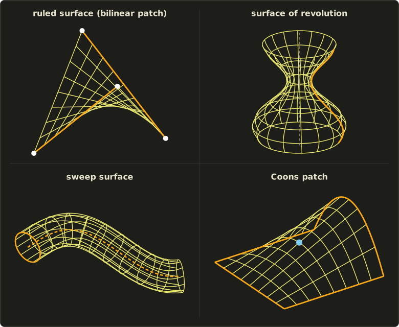
- A ruled surface (線織面) connects two curves and with straight lines: . Every line = const is straight. Cylinders and cones are ruled surfaces, and so is the bilinear patch (双線型曲面), which connects two opposite edges of a quadrilateral. With corners it's the saddle in the picture, a hyperbolic paraboloid, and its center is the average of the corners, . It's ruled in both directions: the lines = const are straight too.
- A surface of revolution (回転面) turns a profile curve around an axis, the "lathe" tool. With a profile in the xy plane rotated about the y axis by : , using the rotation matrix of chapter 5. Vases, glasses, bottles, wheels, chess pieces. The orange curve in the picture is the profile. A profile made of NURBS arcs plus the exact circles of section 8.6 gives an exact NURBS surface.
- A sweep surface (スイープ曲面) moves a cross-section curve along a path curve, keeping it perpendicular to the path. Moving it without turning gives an extrusion (押し出し), a translational sweep; turning it around an axis is again a surface of revolution (a rotational sweep); these are the surfaces of the sweep solids of chapter 7. The general case needs a moving coordinate frame along the path (for example built from the path's tangent, as in the picture), which is why sweeps can twist unexpectedly at tight bends. Pipes, cables, rails, handles, extruded text.
- The Coons patch above is the fourth example.
Trimmed surfaces
A NURBS patch is always a deformed square.
Real parts have holes, rounded cut-outs and edges that follow other surfaces.
A trimmed surface (トリム曲面) keeps the patch but adds trimming curves (トリム曲線) drawn in the parameter square, which mark which part of the square is kept: for example, a closed curve around a hole.
Only the kept region is part of the shape.
Most faces of a CAD solid are trimmed NURBS patches, which is how B-rep models (chapter 7) get faces of arbitrary outline.
Trimming makes tessellation harder, and the boundaries of two neighboring trimmed patches generally don't match exactly in 3D, a source of tiny gaps (the "watertightness" problem) when CAD data is converted to meshes.
Tessellation for rendering
A GPU draws triangles, not patches.
So before rendering, a surface is tessellated (テッセレーション): evaluated at a grid of parameter values, and neighboring points are connected into triangles.
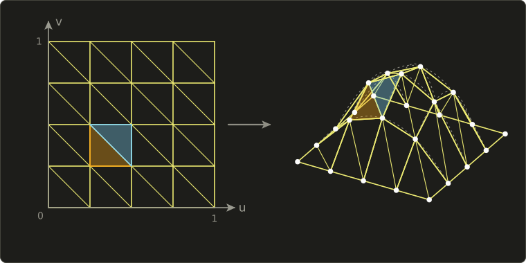
An grid has vertices and triangles: gives 25 vertices and 32 triangles (the picture), gives 289 vertices and 512 triangles.
At each vertex we also evaluate the normal with the cross product above, so the shading is smooth even though the geometry is made of flat triangles.
Adaptive tessellation uses more triangles where the surface bends strongly or is large on screen, and fewer elsewhere.
Then neighboring patches with different levels must agree along their shared edge, or cracks (ひび割れ) open up between them; the usual rule is that both sides of an edge use the same number of segments.
Modern GPUs can do this themselves.
In OpenGL and Vulkan, the tessellation control shader decides how finely to subdivide, a fixed-function tessellator generates the points and triangles, and the tessellation evaluation shader computes for each one, for example with the Bernstein formula of this chapter (Direct3D calls the two programmable stages hull shader and domain shader).
You'll meet these stages in the GLSL series, chapter 15.
Film and animation tools often use subdivision surfaces instead of patches, because they handle any mesh topology; chapter 9 explains them.
8.9 In practice: code and exam points
C++: de Casteljau and Cox–de Boor
Both algorithms fit in a few lines.
This program uses Vec2 and its operators from the Linear Algebra series' linalg.hh, and repeats the worked examples of sections 8.4 and 8.5:
#include "linalg.hh"
#include <cstdio>
#include <vector>

// Linear interpolation between two points: (1 - t) a + t b.
Vec2 lerp(Vec2 a, Vec2 b, float t) { return (1.0f - t) * a + t * b; }

// de Casteljau's algorithm: interpolate neighbors until one point is left.
Vec2 deCasteljau(std::vector<Vec2> p, float t) {
  for (size_t n = p.size() - 1; n > 0; n--) {
    for (size_t i = 0; i < n; i++) {
      p[i] = lerp(p[i], p[i + 1], t);
    }
  }
  return p[0];
}

// Cox-de Boor recursion: B-spline basis function N_{i,p}(t), with 0/0 = 0.
float basisN(int i, int p, float t, const std::vector<float> &knots) {
  if (p == 0) {
    return (knots[i] <= t && t < knots[i + 1]) ? 1.0f : 0.0f;
  }
  float a = 0.0f, b = 0.0f;
  float da = knots[i + p] - knots[i];
  float db = knots[i + p + 1] - knots[i + 1];
  if (da != 0.0f) a = (t - knots[i]) / da * basisN(i, p - 1, t, knots);
  if (db != 0.0f) b = (knots[i + p + 1] - t) / db * basisN(i + 1, p - 1, t, knots);
  return a + b;
}

int main() {
  std::vector<Vec2> bezier = {{0, 0}, {2, 4}, {8, 4}, {8, 0}};
  for (float t : {0.0f, 0.25f, 0.5f, 1.0f}) {
    Vec2 c = deCasteljau(bezier, t);
    printf("Bezier   c(%.2f) = (%g, %g)\n", t, c.x, c.y);
  }

  std::vector<float> knots = {0, 0, 0, 1, 2, 2, 2};
  std::vector<Vec2> ctrl = {{0, 0}, {2, 4}, {6, 4}, {8, 0}};
  float t = 0.5f;
  Vec2 c{};
  printf("N(0.5)  =");
  for (int i = 0; i < 4; i++) {
    float n = basisN(i, 2, t, knots);
    printf(" %g", n);
    c = c + n * ctrl[i];
  }
  printf("\nB-spline c(0.5) = (%g, %g)\n", c.x, c.y);
  return 0;
}
Expected output:
Bezier   c(0.00) = (0, 0)
Bezier   c(0.25) = (2.09375, 2.25)
Bezier   c(0.50) = (4.75, 3)
Bezier   c(1.00) = (8, 0)
N(0.5)  = 0.25 0.625 0.125 0
B-spline c(0.5) = (2, 3)
deCasteljau takes the vector by value on purpose, so it can overwrite its own copy level by level.
basisN is the recursion exactly as written in section 8.5; it's fine for learning, but it recomputes the same lower-degree functions many times, so real libraries evaluate all the nonzero functions of a span together in one triangular loop (or use de Boor's algorithm).
One more detail: with the half-open spans , the very last parameter value ( here) falls into no span, so libraries treat the end of the range as a special case.
A shader function: a point on a cubic Bézier curve
On the GPU, the Bernstein form is the convenient one: no loops, a fixed number of multiplications.
These functions return the position and the tangent of a cubic Bézier curve, which is what you need to bend a strip of vertices along a path (hair, ropes, trails, a curved road) or, inside a tessellation evaluation shader, to place the generated vertices.
// Point on a cubic Bezier curve: Bernstein weights (1-t)^3, 3t(1-t)^2, 3t^2(1-t), t^3.
float3 bezierPoint(float3 p0, float3 p1, float3 p2, float3 p3, float t) {
  float s = 1.0 - t;
  return s * s * s * p0 + 3.0 * s * s * t * p1 + 3.0 * s * t * t * p2 + t * t * t * p3;
}

// Tangent c'(t) = 3 [ (1-t)^2 (p1-p0) + 2t(1-t) (p2-p1) + t^2 (p3-p2) ].
float3 bezierTangent(float3 p0, float3 p1, float3 p2, float3 p3, float t) {
  float s = 1.0 - t;
  return 3.0 * (s * s * (p1 - p0) + 2.0 * s * t * (p2 - p1) + t * t * (p3 - p2));
}
// Point on a cubic Bezier curve: Bernstein weights (1-t)^3, 3t(1-t)^2, 3t^2(1-t), t^3.
vec3 bezierPoint(vec3 p0, vec3 p1, vec3 p2, vec3 p3, float t) {
float s = 1.0 - t;
return s * s * s * p0 + 3.0 * s * s * t * p1 + 3.0 * s * t * t * p2 + t * t * t * p3;
}
// Tangent c'(t) = 3 [ (1-t)^2 (p1-p0) + 2t(1-t) (p2-p1) + t^2 (p3-p2) ].
vec3 bezierTangent(vec3 p0, vec3 p1, vec3 p2, vec3 p3, float t) {
float s = 1.0 - t;
return 3.0 * (s * s * (p1 - p0) + 2.0 * s * t * (p2 - p1) + t * t * (p3 - p2));
}// Point on a cubic Bezier curve: Bernstein weights (1-t)^3, 3t(1-t)^2, 3t^2(1-t), t^3.
float3 bezierPoint(float3 p0, float3 p1, float3 p2, float3 p3, float t) {
float s = 1.0 - t;
return s * s * s * p0 + 3.0 * s * s * t * p1 + 3.0 * s * t * t * p2 + t * t * t * p3;
}
// Tangent c'(t) = 3 [ (1-t)^2 (p1-p0) + 2t(1-t) (p2-p1) + t^2 (p3-p2) ].
float3 bezierTangent(float3 p0, float3 p1, float3 p2, float3 p3, float t) {
float s = 1.0 - t;
return 3.0 * (s * s * (p1 - p0) + 2.0 * s * t * (p2 - p1) + t * t * (p3 - p2));
}
With the control points of section 8.4 (and z = 0) and t = 0.5, bezierPoint returns (4.75, 3, 0) and bezierTangent returns (10.5, 0, 0).
Here every product is a scalar times a vector, so * is right in all three languages; in Slang and HLSL, mul is needed only for products that involve a matrix.
Exam points
- Which points does the curve pass through? Bézier: only the first and last control points. Uniform B-spline: none; clamped (open uniform) B-spline: first and last. Hermite: both end points (and it takes the given tangents there). Catmull–Rom and natural splines: every point. Bicubic Bézier patch: only the four corners.
- Tangents at the ends of a Bézier curve lie along the first and last legs of the control polygon: , . Bézier ↔ Hermite: , .
- Convex hull property: Bézier, B-spline and NURBS (positive weights) curves lie inside the convex hull of their control points, because the weights are non-negative and add up to 1. Catmull–Rom and Hermite curves don't have it.
- Local vs global control: Bézier curves and natural splines are global; B-splines, NURBS and Catmull–Rom splines are local. A cubic B-spline segment depends on 4 control points.
- Degree: a Bézier curve with control points has degree . A B-spline's degree is chosen independently; knots control points degree . Order degree .
- C vs G continuity: means equal tangent vectors, only equal directions. Joining cubic Béziers: collinear gives , and equal legs as well give . The uniform cubic B-spline is , Catmull–Rom ; a repeated knot lowers continuity.
- What NURBS adds: weights and the rational form, computed via homogeneous coordinates and the division by w. Exact conics (the quarter circle with weights ) and projective invariance; Bézier and B-spline curves are special cases. Non-rational curves are only affine invariant.
- Affine invariance: transform the control points, not every curve point.
- Surfaces: tensor-product patches (bicubic Bézier: 16 control points), normal , Coons patch from four boundary curves, ruled surface from straight lines between two curves, surface of revolution and sweep, trimming curves in the domain, tessellation into triangles before rendering.
8.10 Summary
- Parametric curves are the CG standard: easy to generate in order, any shape, in 2D or 3D. Explicit forms can't make closed or vertical curves; implicit forms are good for inside/outside tests.
- The tangent vector gives the direction (shape) and the speed (parameterization). continuity compares derivative vectors, only the geometry: = same tangent direction, = same curvature.
- Cubic pieces are the standard: the lowest degree with inflections, 3D twist and smooth joins. Every curve type is "basis functions times data", or a basis matrix between a row of powers of and a column of points.
- Hermite curves use end points and tangents. Bézier curves use control points with Bernstein weights; de Casteljau's algorithm evaluates and subdivides them by repeated linear interpolation. They interpolate the end points, are tangent to the end legs, stay in the convex hull, are affine invariant and variation diminishing, and have global control.
- B-splines are piecewise polynomials over a knot vector, defined by the Cox–de Boor recursion. They have local control, a degree independent of the number of points, and the uniform cubic B-spline is . Bézier curves are the special case with clamped knots and no inner knots.
- NURBS add weights through homogeneous coordinates: exact circles and other conics, projective invariance, one representation for all CAD geometry.
- Interpolating splines pass through their points: Catmull–Rom (, local, tangents from the neighbors) and natural cubic splines (, global).
- Surfaces: tensor-product Bézier, B-spline and NURBS patches; normals from ; Coons patches from boundaries; ruled surfaces, surfaces of revolution and sweeps; trimmed surfaces for holes; tessellation into triangles (on the GPU in the tessellation stages) for rendering.
8.11 Key terms
| English | 日本語 | Note |
|---|---|---|
| free-form curve / surface | 自由曲線/自由曲面 | shapes defined by control data, not by simple equations |
| explicit / implicit / parametric representation | 陽関数表現/陰関数表現/パラメトリック表現 | , , |
| tangent vector | 接線ベクトル | : direction and speed |
| spline | スプライン | piecewise polynomial curve |
| parametric continuity (C0, C1, C2) | パラメトリック連続性(C0・C1・C2連続) | equal derivative vectors |
| geometric continuity (G1, G2) | 幾何学的連続性(G1・G2連続) | equal tangent direction, equal curvature |
| curvature | 曲率 | how sharply a curve bends |
| Hermite curve | エルミート曲線 | end points plus end tangents |
| basis function / basis matrix | 基底関数/基底行列 | the fixed weights of a curve type |
| Bézier curve | ベジェ曲線 | Bernstein-weighted control points |
| Bernstein polynomial | バーンスタイン多項式 | binomial coefficient times |
| control point / control polygon | 制御点/制御多角形 | the data a designer moves |
| de Casteljau's algorithm | ド・カステリョのアルゴリズム | repeated linear interpolation |
| subdivision | 分割 | splitting a curve into two of the same type |
| convex hull property | 凸包性 | the curve stays inside the hull of its control points |
| affine invariance | アフィン不変性 | transform the control points instead of the curve |
| variation diminishing property | 変動減少性 | no more wiggly than the control polygon |
| global / local control | 大域的制御/局所制御 | how far a moved point's influence reaches |
| degree elevation | 次数上げ | same curve, one more control point |
| B-spline curve | Bスプライン曲線 | piecewise polynomial with automatic continuity |
| knot / knot vector | ノット/ノットベクトル | where the pieces meet |
| uniform / open uniform / non-uniform | 一様/開一様/非一様 | spacing of the knots |
| degree / order | 次数/階数 | order = degree + 1 |
| Cox–de Boor recursion | コックス・ド・ブーアの漸化式 | defines the B-spline basis functions |
| NURBS | NURBS(非一様有理Bスプライン) | weights plus division: exact conics |
| weight | 重み | pulls the curve towards its control point |
| conic section | 円錐曲線 | circle, ellipse, parabola, hyperbola |
| projective invariance | 射影不変性 | projecting the control points projects the curve |
| interpolation / approximation | 補間/近似 | through the points, or only near them |
| Catmull–Rom spline | カトマル・ロム・スプライン | interpolating, C1, local |
| natural cubic spline | 自然3次スプライン | interpolating, C2, global |
| parametric surface / patch | パラメトリック曲面/パッチ | over a parameter square |
| isoparametric curve | アイソパラメトリック曲線(等パラメータ曲線) | u or v held constant |
| tensor-product surface | テンソル積曲面 | the same basis in both directions |
| bicubic Bézier patch | 双3次ベジェ曲面 | 16 control points |
| control net | 制御点網 | the grid of control points of a patch |
| partial derivative / normal vector | 偏微分/法線ベクトル | |
| Coons patch | クーンズ曲面 | filled in from four boundary curves |
| ruled surface | 線織面 | straight lines between two curves |
| bilinear patch | 双線型曲面 | ruled in both directions |
| surface of revolution | 回転面 | a profile turned around an axis |
| sweep surface / extrusion | スイープ曲面/押し出し | a cross-section moved along a path |
| trimmed surface / trimming curve | トリム曲面/トリム曲線 | the kept region marked in the (u, v) domain |
| tessellation | テッセレーション | turning a surface into triangles |
8.12 Challenges
- ★ Evaluate the cubic Bézier curve with control points at with de Casteljau's algorithm, writing down all six intermediate points, then check the result with the Bernstein weights .
- ★★ A quadratic B-spline has the knot vector . How many control points and how many polynomial pieces does it have? Compute all with the Cox–de Boor recursion, check that they add up to 1, and say which control points influence the curve at .
- ★★ For the points , compute the Catmull–Rom tangents at and , the four Bézier control points of the middle segment, and its point at (once with the Hermite weights, once with the Bernstein weights).
- ★★ Evaluate the quarter-circle NURBS of section 8.6 at and via the homogeneous control points, check that both points are at distance 1 from the origin, and compute how far the non-rational curve (all weights 1) is from the circle at the same parameters.
- ★★★ Show that for the quarter-circle NURBS, for every (hint: write and compare numerators with the square of the denominator). Then explain why no polynomial curve can trace an arc of a circle exactly, and what the division by w changes.
Multiple choice
Q1 ★ Which of the following statements about a cubic Bézier curve with control points is correct?
| A | The curve passes through all four control points. |
| B | Its degree is 4, the number of control points. |
| C | Moving changes only the first third of the curve. |
| D | At its start point, the curve is tangent to the line from to . |
| E | The whole curve lies inside the convex hull of the four control points. |
Q2 ★★ Which of the following curves passes through every one of its given points and also has local control (moving one point changes only a limited part of the curve)?
| A | Catmull–Rom spline |
| B | Bézier curve |
| C | uniform cubic B-spline curve |
| D | natural cubic spline |
| E | rational quadratic Bézier curve (NURBS) |
Q3 ★★ Two cubic Bézier segments are joined: the first has the control points , the second , both with . What is the continuity at the joint?
| A | but not |
| B | but not |
| C | but not |
| D | |
| E | not even : the segments don't meet |
8.13 Practical assignment
Design a curve on paper with de Casteljau, check it four ways, and draw an exact circle.
You need graph paper (at least 25 × 17 squares, x from 0 to 24 and y from −4 to 12, with 1 square = 1 unit), a ruler, a pencil, two colored pens, a compass and a calculator.
The control points of the main curve are , , , .
- Control polygon. Draw the four control points and the dashed control polygon. Shade the convex hull lightly with a colored pencil.
- De Casteljau at t = 1/2. Construct the midpoints of the three legs, then of the two new segments, then the final midpoint, with the ruler, and write down all six coordinates. You should end at . Draw the last segment: it's the tangent there.
- More points. Compute and with the Bernstein weights ( and the reverse). Plot the five points and sketch the curve through them, leaving along the first leg and arriving at along the last.
- Subdivision check. From your step 2 construction, write down the control points of the left half of the curve (the left edge of the de Casteljau triangle). Evaluate that half at its own with midpoints. You must get exactly from step 3.
- Hermite check. Compute the Hermite data of the curve, and , and evaluate the Hermite form at with the weights . You must get again.
- A smooth continuation. Add a second cubic segment starting at . Choose so that the joint is , and pick , yourself (for example and ; extend your sheet if needed). Draw its control polygon and sketch it with the other pen. Then mark a second choice of that would make the joint only .
- An exact circle. On a second sheet, draw a circle of radius 4 around the origin with the compass. Take the control points with weights , and compute the rational curve at (homogeneous points, then divide). Plot them in one color. Then compute the same three parameters with all weights 1 and plot them in the other color.
How to check yourself: in step 3, every curve point lies inside the shaded convex hull; step 4 reproduces step 3 exactly; step 5 reproduces step 2 exactly; in step 6, , and your lie on one straight line with exactly halfway (for ), and the alternative lies on the same line but at a different distance; in step 7, all three weighted points have distance 4 from the origin and sit on the compass circle (the middle one at about ), while the unweighted points lie outside it, at about 4.14, 4.24 and 4.14.
Finally, write one sentence for each of the four checks saying which property of this chapter it demonstrates.
コメント(0)
まだコメントはありません。
ログインするとコメント出来ます。