13. Animation 1: Keyframes, Kinematics and Characters
Up to now every picture in this series has been a still: one camera, one scene, one image.
In this chapter things start to move.
An animation is nothing more than many images shown one after another, but deciding what changes between them, and by how much, is a whole craft of its own.
We'll look at how CG animation is organized, how an animator sets a few key poses and lets the computer fill in the rest, why rotations need special care, and how a character is built from a skeleton that moves a skin.
Why does this matter?
Every game character, every animated film and every camera move in a product video is made with the tools of this chapter.
And the math is the math you already know: the transforms and hierarchies of chapter 4 and chapter 5, the Hermite, Bézier and Catmull–Rom curves of chapter 8, and the quaternions of Linear Algebra chapter 13, now with time as the parameter.
For the exam, this chapter covers three syllabus items of area 5: the structure of CG animation (CGアニメーションの構成), keyframe animation (キーフレームアニメーション) and character animation (キャラクタのアニメーション).
The other four items of area 5, physically based, real-time and procedural animation and compositing with live action, are chapter 14.
13.1 Animation is a sequence of frames
A film doesn't really move.
It is a sequence of still pictures, the frames (フレーム, also コマ, koma), shown so quickly that we see motion instead of separate pictures.
That's apparent motion (仮現運動), a property of our vision that chapter 3 (section 3.9) introduced together with flicker; chapter 18 comes back to it with the rest of perception.
The number of frames per second is the frame rate (フレームレート), written fps:
- 24 fps for cinema, since the late 1920s;
- 30 fps (exactly 30000/1001 ≈ 29.97 in the NTSC tradition) and 25 fps (PAL) for television and video;
- 60 fps (or more) for games and VR, where the image must react to the player quickly.
Time and frames
CG animation describes a scene as a function of time in seconds, and the renderer samples it at the frame times.
At a frame rate , frame (counting from 0) shows the moment
Worked example. A shot of 2.5 s at 24 fps has frames; the same shot needs 75 frames at 30 fps and 150 at 60 fps.
Frame 37 at 24 fps is the moment s, and one frame lasts ms.
Keeping the animation as a function of time rather than of frame numbers is what lets the same animation be rendered at 24 fps for a film and at 60 fps for a game.
On ones, twos and threes
Hand-drawn animation rarely draws a new picture for every frame.
Japanese TV anime is usually drawn on twos or on threes (2コマ打ち, 3コマ打ち): each drawing is held for two or three frames of the 24 fps film, so there are 12 or 8 drawings per second.
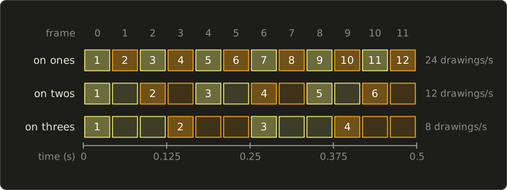
The 2.5 s shot above needs 60 drawings on ones, 30 on twos and 20 on threes.
3D CG is normally computed on ones, because a computed frame is cheap compared with a drawing; anime-style 3D sometimes holds poses on twos or threes on purpose to look hand-drawn.
Sampling in time
Rendering frames is sampling in time, so the sampling theorem of chapter 2 (section 2.6) applies.
Motion that is too fast for the frame rate aliases: the wagon wheel that turns backwards.
The pre-filter in time is motion blur (モーションブラー): average the scene over the time the virtual shutter is open (section 2.3), and fast objects smear along their path instead of jumping.
A 24 fps film with motion blur looks smooth; a 24 fps game without it looks choppy.
13.2 The structure of CG animation
What can change over time
Anything in a scene that is described by a number can be animated:
- transforms: the position, orientation and scale of objects (the modeling transforms of chapters 4 and 5);
- the camera: its position, orientation, focal length or field of view, focus distance;
- lights: position, color, intensity, the cone of a spotlight;
- materials: colors, transparency, texture offsets (a scrolling water texture);
- shape: the vertices themselves, deformed by blend shapes, lattices or a skeleton (sections 13.5 and 13.8);
- any other parameter: the strength of a wind, the number of particles emitted, the visibility of an object.
Each animated number is a channel (チャンネル) or animation curve, a function of time; a walking character easily has a few hundred of them.
The hierarchy: a scene graph
Objects are rarely independent.
A wheel turns on a car that drives through a world; a finger bends on a hand that moves with an arm.
CG software arranges the scene as a tree, the scene graph (シーングラフ) or hierarchy (階層構造): every node has a local transform relative to its parent (親), and its world transform is its parent's world transform times its own local one:
This is exactly the composition of chapter 4 (section 4.3), applied level after level, with the rightmost matrix acting first (Linear Algebra chapter 7).
The payoff for animation is huge: to drive the car you animate one transform, the car's, and the wheels, the driver and the driver's hat follow.
A character's skeleton is the same idea with joints as nodes, and section 13.6 works through it with numbers.
The production flow
A CG film is made in a long chain of stages, and animation sits in the middle of it:
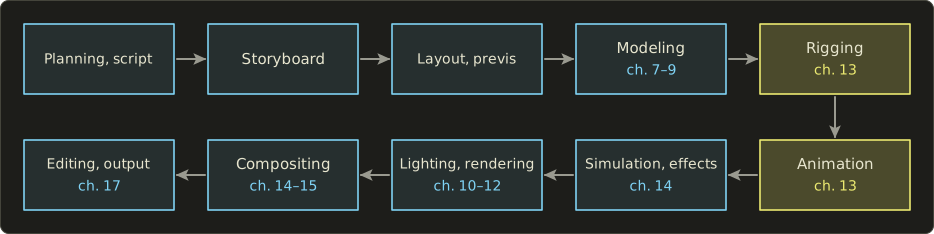
- Planning and script (企画, シナリオ): the story.
- Storyboard (絵コンテ, ekonte): a drawing for each shot, with camera framing, action and timing notes. In Japanese animation the 絵コンテ is the central planning document.
- Layout and previs (レイアウト, プリビズ): rough 3D versions of the shots that fix the camera, the positions of the characters and the timing of each cut.
- Modeling (chapters 7–9) and rigging (section 13.8): the characters and props are built and given controls.
- Animation: this chapter. The animators pose the rigs over time.
- Simulation and effects (chapter 14): cloth, hair, fluids, destruction, computed from the animated motion.
- Lighting and rendering (chapters 10–12).
- Compositing (chapters 14 and 15): the rendered layers, and live-action footage, are combined into the final images.
- Editing and output: cutting, sound, and the final file or film (output devices and recording media are in chapter 17).
A game shares the first half (assets, rigs, animation clips), but the second half happens on the player's machine every frame; chapter 14 covers real-time animation.
Four ways to make motion
Who, or what, decides the values of the channels?
| Method | Who decides the motion | Strengths | Weaknesses | Chapter |
|---|---|---|---|---|
| keyframe animation | an animator sets key poses, the computer interpolates | full artistic control, stylized motion | labor-intensive, hard to make physically right | 13 |
| motion capture | a real performer, measured | realistic, fast for large amounts | needs cleanup, hard to exaggerate, limited by the actor | 13 |
| procedural animation | rules and functions (noise, flocking, expressions) | huge numbers of objects, endless variation | hard to direct in detail | 14 |
| physically based animation | simulation of physical laws | believable cloth, fluids, collisions | expensive, hard to direct | 14 |
Real productions mix them: a keyframed character with captured body motion, simulated hair and procedurally animated background crowds.
13.3 Keyframe animation
Keys and in-betweens
In traditional animation, a lead animator draws the important poses, the key frames (原画, genga), and assistants draw the in-betweens (動画, dōga) between them; making the in-betweens is in-betweening (中割り, nakawari).
Keyframe animation (キーフレームアニメーション) moves the second job to the computer.
The animator sets keys (キー): pairs of a time and a value for a channel.
The computer computes the value at every other frame by interpolation (補間).
A ball that rises and falls might need only three keys for its height, while the computer makes the 22 frames in between.
Function curves and the graph editor
Each channel, drawn as value against time, is a function curve (ファンクションカーブ, Fカーブ, F-curve), and the tool that shows and edits these curves is the graph editor (グラフエディタ).
Reading a function curve is a core skill:
- the height of the curve is the value;
- the slope is the speed: a steep curve is fast motion, a flat curve is a hold;
- a kink (a sudden change of slope) is a sudden change of speed, a jolt;
- the curvature is the acceleration.
That's why the continuity classes of chapter 8 (section 8.2) matter here: a curve has no jolts in speed, a curve has continuous acceleration as well.
Step, linear and smooth interpolation
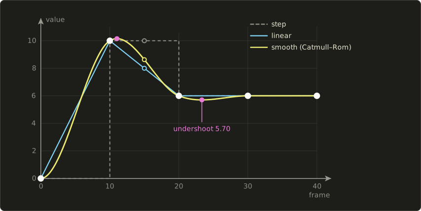
Take one channel with five keys, (frame, value) = (0, 0), (10, 10), (20, 6), (30, 6), (40, 6): something rises to 10, falls back to 6 and stays there.
Step interpolation (ステップ補間, also constant): hold each key's value until the next key.
The motion jumps; animators use it while blocking a shot (posing the key poses only) and for things that really do switch, like a light being turned on.
Linear interpolation (線型補間): a straight line between neighboring keys,
At frame 15, and .
The curve is continuous but has kinks at the keys: the speed changes instantly, which looks mechanical.
Smooth interpolation: a cubic Hermite segment between neighboring keys (chapter 8, section 8.3).
Its tangents are the Catmull–Rom choice of section 8.7: the slope at a key is the slope of the line through its two neighbors.
Because keys are rarely evenly spaced in time, the slope is measured per frame,
and the Hermite curve on the segment uses the tangents and with , because the Hermite parameter runs from 0 to 1 while runs over frames.
At the first and last key, which have only one neighbor, we set the slope to 0 here (a flat start and end).
Worked example. The slopes are , , , and per frame.
On the segment from frame 10 to 20, , so the tangents are and .
At frame 15 () the Hermite weights are (chapter 8):
Step gives 10, linear 8, smooth 8.625.
Overshoot and tangent control
Look at the smooth curve around frame 23.
On the segment from frame 20 to 30 both keys have the value 6, but the tangent at frame 20 is (the curve arrives falling), and the one at frame 30 is 0:
(using ).
is largest at , where it equals , so the value dips to at frame 23.3.
The object that should hold still at 6 sinks below it first: an undershoot.
Likewise, the slope at the peak key (frame 10) is , not 0, so the curve keeps rising past the key, to about 10.15.
This overshoot (オーバーシュート) is the price of an interpolating spline without the convex hull property (section 8.7).
Animation tools give the animator control over it:
- flat or clamped tangents: a key that is a peak, a valley or a hold gets slope 0, so the curve never passes it (many tools have an "auto clamped" default for this);
- broken tangents: different in and out tangents at one key, for a sudden change like a ball hitting the floor;
- tangent handles: the in and out tangents are drawn as handles you drag, exactly the Hermite tangents or the inner Bézier control points of section 8.4, with "weighted" handles also changing the tangent's length.
Overshoot isn't always a bug.
A deliberate small overshoot that settles back is the classic "follow-through" of animation; what animators hate is the accidental kind.
Ease-in and ease-out
Real objects don't start or stop instantly: a door opened by hand speeds up and then slows down.
Starting slowly is ease-in (イーズイン, also slow-in) and stopping slowly is ease-out (イーズアウト, slow-out); "slow in and slow out" is one of the classic principles of Disney animation.
For a move from 0 to 1 over the normalized time , the standard cubic is the smoothstep function
It is nothing new: it is the Hermite basis function of chapter 8, a Hermite segment from 0 to 1 with both tangents 0, the same curve chapter 11 used to smooth value noise.
Its speed is 0 at both ends and in the middle, so the peak speed is 1.5 times the average.
Worked example. A door opens 90° in one second, 24 frames.
With linear motion every frame turns it .
With smoothstep:
| frame | u | s(u) | angle |
|---|---|---|---|
| 0 | 0 | 0 | 0° |
| 6 | 0.25 | 3(0.0625) − 2(0.015625) = 0.15625 | 14.06° |
| 12 | 0.5 | 0.5 | 45° |
| 18 | 0.75 | 0.84375 | 75.94° |
| 24 | 1 | 1 | 90° |
The first frame turns it only , the frames in the middle about each (peak speed per second), and it settles gently into 90°.
Animators draw this as a spacing chart: one tick per frame along the motion, ticks close together where the motion is slow.
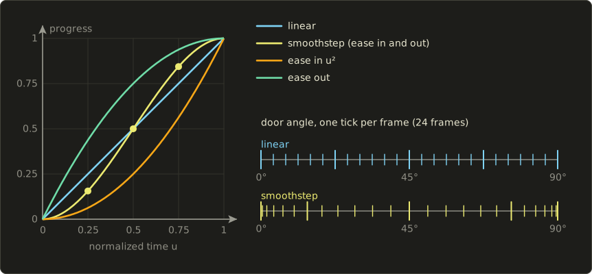
Other common easing curves are ease-in only, , ease-out only, , and their cubic and higher versions.
Bézier curves for timing
Many tools describe the timing of one segment as a cubic Bézier curve in the (time, value) plane, from to with two handles.
The CSS transition ease-in-out of every web browser is the Bézier curve with the inner control points and .
Both coordinates are cubics in the curve parameter :
To find the progress at time , the program first solves for (with a few Newton or bisection steps), then evaluates .
Worked example, : gives , and then .
So after a quarter of the time, this ease has done 12.9 % of the move, a slower start than smoothstep's 15.6 %.
Path and timing
For something that moves through space, like a camera flying along a road, it's convenient to separate where it goes from when it gets there:
- the motion path (モーションパス): a space curve through the places it should pass, usually a Catmull–Rom or Bézier spline (chapter 8);
- the timing: a function curve that gives the distance traveled along the path as a function of time, with its own easing.
The catch: a spline's own parameter does not measure distance.
Take the Hermite curve of chapter 8, section 8.3, from to .
At it is at , , , and , and the chords between these points have the lengths
Equal steps of cover distances between 2.40 and 3.07: a camera moved by at a constant rate would change its speed by more than a quarter for no reason.
The fix is arc-length parameterization (弧長パラメータ化): describe the curve by the distance along it.
Few curves have a closed formula for that, so programs build a table:
- Sample the curve at many values of and add up the chord lengths: here the cumulative lengths are 0, 3.07, 5.83, 8.24, 10.68.
- To place the object at distance , find the interval of the table that contains it and interpolate linearly inside it.
The total, 10.68, is an approximation of the true arc length, 10.89; chords are always a little shorter than the curve, and 8 chords give 10.84 already.
Halfway along, , lies in the second interval: of the way, so (exact: 0.4565), not 0.5.
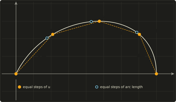
With the table, the timing curve says how far along the path the object is, and the path says where that is.
That's how a camera can follow a winding road at a steady 50 km/h, or ease into a stop exactly at a marked spot.
13.4 Interpolating rotations
Positions, colors and most parameters interpolate perfectly well channel by channel.
Orientations don't, and the reason is worth understanding.
Euler angles, channel by channel
Animation tools usually show a rotation as three Euler angles (chapter 5, section 5.3), one function curve each, because that's easy to read and edit.
Interpolating the three angles separately has the three problems that Linear Algebra chapter 13 (section 13.1) shows with numbers:
- the path between two orientations depends on the rotation order and is generally not the shortest turn;
- angles wrap around: from 170° to −170° is a 20° turn, but the numbers say 340° the other way;
- near gimbal lock (ジンバルロック), when the middle rotation reaches 90° and two axes line up, a small change of orientation needs a huge jump in the angles, and the curves spike.
Tools therefore offer an "Euler filter" that removes the 360° jumps from the curves, and they let the animator switch a joint to quaternion interpolation.
Why not interpolate the matrices?
A rotation matrix is just nine numbers, so why not blend them?
Take the 2D rotations by 0° and 90° (the upper-left part of chapter 4's matrices) and blend halfway:
Its columns have length and its determinant is .
It is the rotation by 45° times a scaling by 0.707: the object turns the right amount, but shrinks to 71 % of its size in the middle of the move.
Between 0° and 180° it's worse: , and the object collapses to a single point.
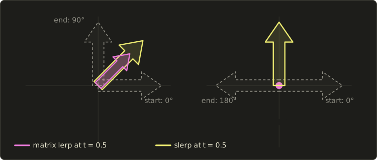
In general, a weighted sum of rotation matrices is not a rotation: the rotations form a curved set, and averaging cuts through its inside.
Renormalizing the columns afterwards helps but doesn't give constant speed, and the 180° case has nothing left to renormalize.
Quaternion slerp
The standard answer is the unit quaternion (クォータニオン, 四元数) from Linear Algebra chapter 13: a rotation by about the unit axis is
written , and unit quaternions are points on the 4D unit sphere.
Spherical linear interpolation, slerp (球面線型補間), walks along that sphere at constant speed (Ken Shoemake brought it to computer animation in 1985):
(if , use , the same rotation, to take the short way round; the linear algebra chapter explains why).
Worked example. A turret is keyed at 30° about z at one key and at 110° about z at the next.
and .
Their dot product is , so , half the 80° between the two keys.
At both weights are :
which is : a rotation by 70°, exactly halfway between 30° and 110°.
At the weights are and , which gives , 50°: a quarter of the way, at constant speed.
nlerp (normalized lerp) blends the four numbers and normalizes.
At it gives , a rotation by 49.37° instead of 50°; at it agrees with slerp.
For neighboring keys of an animation, a fraction of a degree is invisible and nlerp is cheaper, which is why many game engines use it; for large turns slerp's constant speed matters.
Slerp between two keys is the rotation version of linear interpolation: it has kinks in angular speed at the keys.
Smooth curves through many orientations (the rotation version of Catmull–Rom) exist too, for example Shoemake's squad, built from nested slerps like de Casteljau's algorithm of chapter 8.
In practice
Animators keep editing Euler curves, while the data that ships to a game engine usually stores quaternion keys.
The glTF 2.0 file format (chapter 9) is a good example: its animation samplers offer exactly the three interpolations of this section, STEP, LINEAR and CUBICSPLINE (Hermite segments with stored tangents), and the specification says that LINEAR on a rotation means slerp of the quaternions, which it stores in order.
You'll read glTF files yourself in the OpenGL series, chapter 13.
Here are the key interpolation of section 13.3, the door's smoothstep, and the slerp of the worked example in C++, with Quat and slerp from the Linear Algebra series' linalg.hh:
#include <cstdio>
#include <vector>
#include "linalg.hh"

enum class Interp { Step, Linear, Smooth };

struct Key {
  float time;  // in frames
  float value;
};

// Catmull–Rom slope at key i (value per frame); flat at the first and the last key.
float keySlope(const std::vector<Key> &k, size_t i) {
  if (i == 0 || i + 1 == k.size()) return 0.0f;
  return (k[i + 1].value - k[i - 1].value) / (k[i + 1].time - k[i - 1].time);
}

// Value of an animation channel at time t (keys sorted by time).
float evaluate(const std::vector<Key> &k, float t, Interp mode) {
  if (t <= k.front().time) return k.front().value;
  if (t >= k.back().time) return k.back().value;
  size_t i = 0;
  while (k[i + 1].time < t) ++i; // the segment k[i] .. k[i + 1] contains t
  float d = k[i + 1].time - k[i].time;
  float s = (t - k[i].time) / d; // 0 .. 1 inside the segment
  float v0 = k[i].value, v1 = k[i + 1].value;
  switch (mode) {
  case Interp::Step: return v0;
  case Interp::Linear: return v0 + s * (v1 - v0);
  case Interp::Smooth: {
    float s2 = s * s, s3 = s2 * s; // Hermite basis functions (chapter 8)
    float h0 = 2 * s3 - 3 * s2 + 1, h1 = -2 * s3 + 3 * s2, h2 = s3 - 2 * s2 + s, h3 = s3 - s2;
    return h0 * v0 + h1 * v1 + h2 * keySlope(k, i) * d + h3 * keySlope(k, i + 1) * d;
  }
  }
  return v0;
}

float smoothstep01(float u) { return u * u * (3.0f - 2.0f * u); }

int main() {
  std::vector<Key> keys = {{0, 0}, {10, 10}, {20, 6}, {30, 6}, {40, 6}};
  for (float t : {5.0f, 15.0f, 23.3333f}) {
    printf("frame %5.2f: step %g, linear %g, smooth %.4g\n", t, evaluate(keys, t, Interp::Step),
           evaluate(keys, t, Interp::Linear), evaluate(keys, t, Interp::Smooth));
  }
  for (int f = 0; f <= 24; f += 6) {
    printf("door at frame %2d: %.4g degrees\n", f, 90.0f * smoothstep01(f / 24.0f));
  }
  Quat a = Quat::fromAxisAngle({0, 0, 1}, 30.0f * 3.14159265f / 180.0f);
  Quat b = Quat::fromAxisAngle({0, 0, 1}, 110.0f * 3.14159265f / 180.0f);
  Quat m = slerp(a, b, 0.5f);
  printf("slerp(30, 110, 0.5) = (%.4f, %.4f, %.4f, %.4f)\n", m.w, m.x, m.y, m.z);
  return 0;
}
frame  5.00: step 0, linear 5, smooth 4.625
frame 15.00: step 10, linear 8, smooth 8.625
frame 23.33: step 6, linear 6, smooth 5.704
door at frame  0: 0 degrees
door at frame  6: 14.06 degrees
door at frame 12: 45 degrees
door at frame 18: 75.94 degrees
door at frame 24: 90 degrees
slerp(30, 110, 0.5) = (0.8192, 0.0000, 0.0000, 0.5736)
Exam points
- Keyframe animation: the animator sets keys, the computer makes the in-betweens (中割り) by interpolation.
- Step holds, linear has kinks in speed at the keys, smooth (Hermite with Catmull–Rom tangents) passes through every key with continuous speed but can overshoot; flat or clamped tangents prevent that.
- Ease-in/ease-out: zero speed at the ends; smoothstep is the Hermite , with peak speed 1.5 times the average.
- A spline's parameter is not distance: constant speed along a path needs arc-length parameterization.
- Don't interpolate Euler angles or matrix entries for general rotations: Euler angles give wrong paths and gimbal lock, matrix blending shrinks (0° to 90°: scale 0.707) or collapses (0° to 180°). Use quaternion slerp (constant speed) or nlerp (cheaper, nearly the same for small steps).
13.5 Shape interpolation and deformation
Keys don't have to be numbers like an angle.
A key can be a whole shape.
Shape interpolation and morphing
If two shapes and have the same number of vertices and vertex of corresponds to vertex of , every vertex can simply be interpolated:
This is shape interpolation (形状補間), and an animation that turns one shape into another this way is morphing (モーフィング).
The hard part is not the formula but the correspondence (対応付け): which vertex of a cat matches which vertex of a teapot?
If the shapes are built from the same base mesh (a face in two expressions), the correspondence is free; between unrelated models it has to be made, by remeshing both or by matching features by hand.
Morphing between two images instead of two meshes, with warping plus cross-dissolve, is a 2D image-processing technique: chapter 15 covers it, and chapter 12 met it as image-based rendering.
Blend shapes
Blend shapes (ブレンドシェイプ), also morph targets (モーフターゲット) or shape keys, generalize this to many shapes at once.
An artist sculpts a neutral base mesh and several targets with the same vertices: smile, jaw open, blink, frown…
Each target gets a weight , an animated channel, and the result adds up the differences from the base:
Worked example. One vertex at the corner of a mouth: base , "smile" target , "jaw open" target , weights 0.5 and 0.8.
The deltas are and , so
A half smile with the mouth mostly open: the corner moves out (x) and slightly up from the smile, and down from the jaw.
Because the deltas add, the targets combine freely; a weight above 1 exaggerates a shape, a negative weight inverts it.
Combinations that don't add up well (a smile while the jaw is open often looks wrong) get extra corrective shapes that are switched on only when both weights are high.
Blend shapes are the workhorse of facial animation (section 13.8) and are supported directly by glTF and every game engine.
Path animation
Path animation (パスアニメーション) moves an object along a motion path (section 13.3) and usually also orients it along the path: the object's forward axis follows the path's tangent (chapter 8), and a chosen up vector fixes the roll, building the orientation exactly like the lookAt construction of chapter 5 with the tangent as the viewing direction.
A car on a road, a train on rails, a camera on a dolly track and a fish swimming on a curve are all path animations.
Free-form deformation
Free-form deformation (FFD, フリーフォームデフォメーション; Sederberg and Parry, 1986) deforms an object by deforming the space around it.
The object is embedded in a lattice (ラティス) of control points; every point of the object gets local coordinates from 0 to 1 inside the lattice, and its deformed position is a Bézier volume of the control points, built with the Bernstein polynomials of chapter 8 (section 8.4):
As long as the control points sit on their regular grid, gives back the original point; when the animator moves a control point, everything near it moves smoothly.
Worked example in 2D, with a 3 × 3 lattice (quadratic in both directions, , , ) over the rectangle from to .
The control points are at and .
Move only the center one, , from up to .
Every point moves by times that displacement :
- the center , with : in both directions, so it moves up by , to ;
- the point , with : , so it moves up by ;
- points on the border ( or equal to 0 or 1) don't move, because is 0 there.
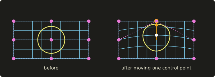
The deformation is smooth and needs no knowledge of the object's mesh, so it works on anything with points: a character's belly that breathes, a cartoon squash-and-stretch, a car bending in a crash.
DCC tools call it a lattice deformer; related deformers bend, twist or taper an object, or deform it by a coarse cage mesh around it.
13.6 Skeletons and forward kinematics
Skeletons, bones and joints
Characters are animated through a skeleton (スケルトン, 骨格): a hierarchy of joints (関節, ジョイント) connected by bones (ボーン).
It is the scene graph of section 13.2 with joints as nodes, usually rooted at the hips, the root (ルート), whose transform moves the whole character through the world.
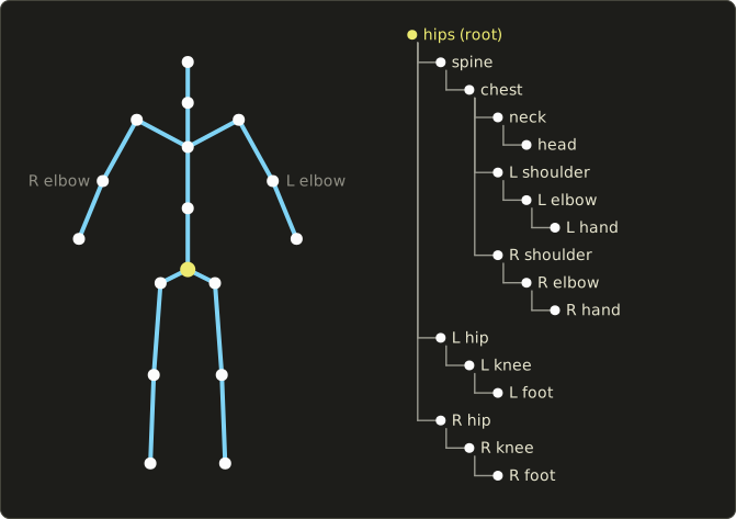
Each joint stores a fixed offset from its parent (the bone length and direction in the rest pose) and an animated rotation.
How many independent rotations a joint allows is its number of degrees of freedom (自由度, DOF):
- a hinge joint like the elbow or the knee: 1 DOF, a bend about one axis;
- a ball joint like the shoulder or the hip: 3 DOF;
- the root: 6 DOF, 3 for position and 3 for orientation.
Joints also get joint limits (可動域): a knee bends one way only, from about 0° to 150°.
A typical game character has 30 to 100 joints, a film character with fingers and facial joints a few hundred.
Forward kinematics
Forward kinematics (フォワードキネマティクス, FK, 順運動学) computes the position of every joint from the joint angles, going down the hierarchy from the root: each joint's world transform is its parent's world transform times its own offset and rotation.
The last joint of a chain, the one that should reach somewhere (a hand, a foot, a fingertip), is the end effector (エンドエフェクタ).
The simplest example is a planar arm with two links: an upper arm of length that turns by at the shoulder, and a forearm of length that turns by relative to the upper arm at the elbow:
Applied to the origin, it gives
The forearm's direction is , because its rotation is relative to its parent: turning the shoulder carries the whole forearm with it.
Worked example. , , , :
FK is what the animator does when posing joint by joint ("rotate the shoulder 30°, then the elbow 45°"), and it's also what every engine does each frame to turn the animated joint rotations into world matrices.
It's natural for swinging motion like a tail or an arm in a walk, but awkward for contact: putting the hand exactly on a door handle by turning shoulder and elbow angles is trial and error.
Here is FK down a joint array with linalg.hh (parents stored before their children, so one pass from the start is enough), together with the analytic IK of the next section:
#include <cmath>
#include <cstdio>
#include <initializer_list>
#include "linalg.hh"

// One joint of a chain: its parent (-1 for the root), the offset from the parent's joint in the
// parent's frame, and the animated rotation about z.
struct Joint {
  int parent;
  Vec3 offset;
  float angle;
};

// Forward kinematics: world = parent's world * T(offset) * Rz(angle).
// Parents come first in the array.
void forwardKinematics(const Joint *joints, int count, Mat4 *world) {
  for (int i = 0; i < count; ++i) {
    Mat4 local = translate(joints[i].offset) * rotateZ(joints[i].angle);
    world[i] = joints[i].parent < 0 ? local : world[joints[i].parent] * local;
  }
}

// Analytic two-link IK in the plane.
// Returns false (and stretches towards the target) if the target is out of reach.
bool solveTwoLink(float l1, float l2, float x, float y, bool elbowDown,
                  float &theta1, float &theta2) {
  float c2 = (x * x + y * y - l1 * l1 - l2 * l2) / (2.0f * l1 * l2); // law of cosines
  bool reachable = c2 >= -1.0f && c2 <= 1.0f;
  c2 = std::fmax(-1.0f, std::fmin(1.0f, c2));
  theta2 = (elbowDown ? 1.0f : -1.0f) * std::acos(c2);
  theta1 = std::atan2(y, x) - std::atan2(l2 * std::sin(theta2), l1 + l2 * std::cos(theta2));
  return reachable;
}

int main() {
  const float deg = 3.14159265f / 180.0f;
  Joint arm[3] = {
    {-1, {0, 0, 0}, 30 * deg}, // shoulder
    {0, {3, 0, 0}, 45 * deg},  // elbow, 3 units along the upper arm
    {1, {2, 0, 0}, 0},         // hand (end effector), 2 units along the forearm
  };
  Mat4 world[3];
  forwardKinematics(arm, 3, world);
  for (int i = 1; i < 3; ++i) {
    Vec4 p = world[i] * Vec4{0, 0, 0, 1};
    printf("joint %d at (%.3f, %.3f)\n", i, p.x, p.y);
  }
  for (bool down : {true, false}) {
    float t1, t2;
    bool ok = solveTwoLink(3, 2, 3.1157f, 3.4319f, down, t1, t2);
    printf("IK %s: theta1 = %.2f, theta2 = %.2f (%s)\n", down ? "elbow down" : "elbow up",
           t1 / deg, t2 / deg, ok ? "reachable" : "out of reach");
  }
  float t1, t2;
  bool ok = solveTwoLink(3, 2, 6, 0, true, t1, t2);
  printf("IK (6, 0): theta1 = %.2f, theta2 = %.2f (%s)\n", t1 / deg, t2 / deg,
         ok ? "reachable" : "out of reach");
  return 0;
}
joint 1 at (2.598, 1.500)
joint 2 at (3.116, 3.432)
IK elbow down: theta1 = 30.00, theta2 = 45.00 (reachable)
IK elbow up: theta1 = 65.53, theta2 = -45.00 (reachable)
IK (6, 0): theta1 = 0.00, theta2 = 0.00 (out of reach)
13.7 Inverse kinematics
Inverse kinematics (インバースキネマティクス, IK, 逆運動学) goes the other way: given where the end effector should be, find the joint angles.
The animator drags the hand to the door handle, or pins a foot to the ground, and the solver bends the elbow or the knee to match.
Games use IK every frame to put feet on uneven ground, hands on a ladder or a weapon, and a head turned towards what the character looks at.
The analytic two-link solution
For the two-link arm, IK can be solved exactly with school geometry.
The shoulder, the elbow and the target form a triangle with sides , and the distance to the target .
The law of cosines (余弦定理) gives the elbow angle:
(The inner angle of the triangle at the elbow is , and is the same equation.)
Then the shoulder angle is the direction to the target minus the angle that the bent arm makes with that direction:
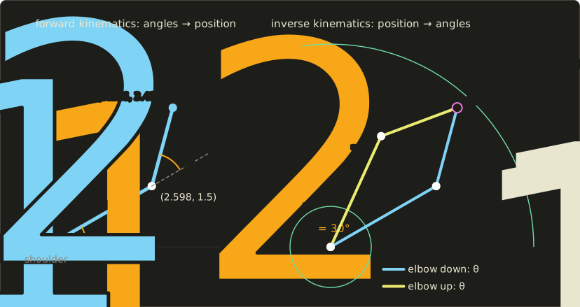
Worked example. Ask for the hand position of the FK example, , with , .
, so
With : and , so .
We got back the angles we started with.
With the second atan2 changes sign, and : the same hand position with the elbow on the other side.
How many solutions?
The worked example shows the typical situation, and the formula for shows all of them:
- Out of reach: (target farther than ) or (closer than ). There is no solution; a solver usually stretches the arm straight towards the target. Here the reachable region is the ring ; the target is outside it.
- On the boundary ( or ): exactly one solution, the arm fully stretched or fully folded.
- Inside the ring: two solutions, elbow up and elbow down. A real elbow can only bend one way, so the joint limit picks one.
- With and the target at the shoulder, there are infinitely many.
In 3D, the elbow of a two-link arm can be anywhere on a circle around the shoulder–target line, so the animator gives a pole vector that says which way the elbow (or knee) should point.
You'll write the 2D solver for a fighting game's legs in OpenGL chapter 30 and the 3D version with a pole vector for a character's arms in OpenGL chapter 36.
Longer chains (a spine, a tail, a robot arm with six joints) have more degrees of freedom than the target needs: they are redundant, and there are infinitely many solutions.
Then the solver needs extra goals: stay close to the current pose, respect the joint limits, keep the motion smooth.
Iterative solvers: CCD
For chains without a closed formula, IK is solved by small steps.
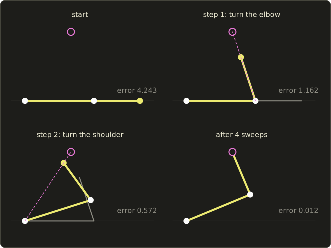
The simplest method is cyclic coordinate descent (CCD): go through the joints from the last one to the root, and turn each joint so that the line from it to the end effector points straight at the target; repeat the sweep until the effector is close enough.
Worked example. Our arm (, ) starts straight along x, so the hand is at ; the target is , at distance from the hand.
- Elbow (at ): the hand is in the direction , 0°; the target is in the direction , . Turn the elbow by 108.43°: the hand moves to , now 1.162 from the target.
- Shoulder (at the origin): the hand is at , the target at . Turn the shoulder by 17.60°: the hand moves to , 0.572 from the target.
| after sweep | θ1 | θ2 | hand | error |
|---|---|---|---|---|
| 1 | 17.60° | 108.43° | (1.683, 2.524) | 0.572 |
| 2 | 21.20° | 94.73° | (1.922, 2.884) | 0.140 |
| 3 | 22.19° | 91.39° | (1.977, 2.966) | 0.041 |
| 4 | 22.49° | 90.42° | (1.993, 2.990) | 0.012 |
The exact answer (from the formula: , so and ) is approached quickly.
CCD is simple and works for any chain length, but it tends to curl the joints near the end first, and its result depends on the order of the joints.
A popular newer method, FABRIK (Aristidou and Lasenby, 2011), moves the joint positions back and forth along the chain instead of turning angles and often looks more natural.
The Jacobian idea
A more general approach linearizes FK: for small angle changes , the end effector moves by
where the Jacobian (ヤコビ行列) holds the partial derivatives of the effector position with respect to each joint angle, one column per joint.
For a rotation joint in the plane at , its column is the effector's velocity when that joint turns, perpendicular to the line from the joint to the effector: .
In the FK pose above, the shoulder's column is and the elbow's .
To move the hand by a small towards the target, solve for with the inverse (Linear Algebra chapter 10), or with the transpose or the pseudo-inverse when isn't square, take the small step, recompute , and repeat.
The determinant of this is , which is .
When the arm is straight (), it is 0: the arm can't move its hand along its own length, is singular, and naive solvers jitter. Real solvers add damping (damped least squares) for that.
FK and IK together
Rigs usually offer both on one limb with an FK/IK switch: FK for free swinging (arms in a walk), IK for contact (hands on a table, feet on the floor), with a blend between the two for the moment a hand lets go.
13.8 Skinning, rigging and facial animation
A skeleton is invisible.
What we see is a mesh, the skin, which has to follow the bones: that's skinning (スキニング), and binding a mesh to a skeleton is called binding (バインド).
Rigid binding
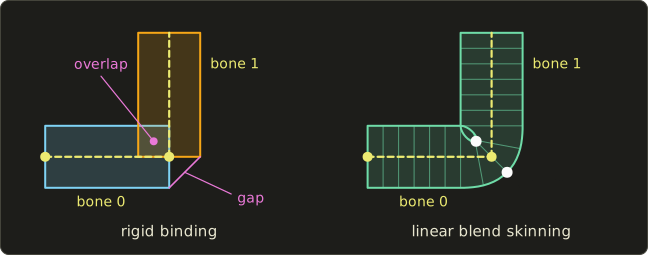
The simplest way is to attach each vertex to exactly one bone, rigid binding (剛体バインド, also rigid skinning).
Each piece of the mesh then moves rigidly with its bone, like the parts of a robot or a puppet.
At a joint it breaks: on the outside of a bend the pieces open a gap, on the inside they overlap.
That's fine for robots or for characters that are separate parts by design (the blocky soldier of OpenGL chapter 36), but not for skin.
Linear blend skinning
Linear blend skinning (LBS, リニアブレンドスキニング; also called smooth skinning or skeletal subspace deformation) lets each vertex follow several bones with weights (ウェイト).
The mesh is modeled in a rest pose, the bind pose (バインドポーズ), in which each bone has the world matrix .
In the animated pose bone has the world matrix .
The vertex is first carried into each bone's local frame by , moved with the bone by , and the results are averaged:
is the inverse bind matrix (逆バインド行列), computed once; is the bone's skinning matrix, which is the identity while the character stands in the bind pose, so the mesh stays where it was modeled.
Vertices far from a joint get weight 1 on their own bone; near a joint the weights fade smoothly from one bone to the next.
Real-time engines usually allow up to 4 influences per vertex (glTF stores them as JOINTS_0 and WEIGHTS_0, four of each).
Painting these weights on the mesh is weight painting (ウェイトペイント), a big part of a rigger's job.
Worked example in 2D, with the homogeneous 3 × 3 matrices of chapter 4.
Bone 0 (the upper arm) runs from to , bone 1 (the forearm) from on, and the arm is a tube of radius 0.5.
Bind pose: , .
Pose: the upper arm stays, the forearm bends up by 90° at the elbow: , .
Take the vertex on the outside of the elbow, , with weights .
- Bone 0: , so .
- Bone 1: ; sends to , giving ; gives .
- Blend: .
The vertex lies between the two rigid positions, and the gap is gone.
But measure its distance from the elbow : instead of the tube's radius 0.5.
The inside vertex lands at , also 0.354 from the elbow.
The elbow has become thinner: averaging two rotated copies of a point pulls it towards the center of rotation, exactly like the matrix lerp of section 13.4.
The candy-wrapper artifact
The same effect is much worse when a joint twists about the bone's own axis, like a forearm turning a doorknob.
Let bone 1 twist by about the x axis, and take a vertex of the tube at the joint, , with weights 0.5 and 0.5.
Bone 1 moves it to , and the blend is
For that's , radius 0.354; for it's , radius 0: every vertex of that ring collapses onto the bone.
The tube is pinched like the twisted ends of a wrapped candy, hence the name candy-wrapper artifact (キャンディラッパー現象).

The fixes:
- more bones: split the forearm into a few twist bones that share the twist, so no joint turns by much;
- corrective blend shapes that restore the volume in bad poses;
- dual quaternion skinning (デュアルクォータニオンスキニング; Kavan and others, 2007): blend the bones' rigid transforms as dual quaternions, which blend rotations properly like nlerp does, instead of blending matrices. It keeps the radius, at a slightly higher cost, and has its own artifact (a small bulge at bent joints). Part 2 treats it in depth.
On the GPU
Skinning runs in the vertex shader: the engine computes the skinning matrices for the current pose on the CPU (FK of section 13.6, then times the inverse bind matrices), uploads them as an array, the matrix palette, and each vertex blends its four:
struct JointPalette {
  float4x4 skinning[64]; // S_j = W_j * inverse(B_j) for every joint
};
ConstantBuffer<JointPalette> palette;

// Linear blend skinning of one position with four joint indices and weights (summing to 1).
float3 skinPosition(float3 position, uint4 joints, float4 weights) {
  float4 p = float4(position, 1.0);
  float4 r = weights.x * mul(palette.skinning[joints.x], p)
           + weights.y * mul(palette.skinning[joints.y], p)
           + weights.z * mul(palette.skinning[joints.z], p)
           + weights.w * mul(palette.skinning[joints.w], p);
  return r.xyz;
}layout(set = 0, binding = 1) uniform JointPalette {
mat4 skinning[64]; // S_j = W_j * inverse(B_j) for every joint
};
// Linear blend skinning of one position with four joint indices and weights (summing to 1).
vec3 skinPosition(vec3 position, uvec4 joints, vec4 weights) {
vec4 p = vec4(position, 1.0);
vec4 r = weights.x * (skinning[joints.x] * p)
+ weights.y * (skinning[joints.y] * p)
+ weights.z * (skinning[joints.z] * p)
+ weights.w * (skinning[joints.w] * p);
return r.xyz;
}struct JointPalette {
float4x4 skinning[64]; // S_j = W_j * inverse(B_j) for every joint
};
ConstantBuffer<JointPalette> palette;
// Linear blend skinning of one position with four joint indices and weights (summing to 1).
float3 skinPosition(float3 position, uint4 joints, float4 weights) {
float4 p = float4(position, 1.0);
float4 r = weights.x * mul(palette.skinning[joints.x], p)
+ weights.y * mul(palette.skinning[joints.y], p)
+ weights.z * mul(palette.skinning[joints.z], p)
+ weights.w * mul(palette.skinning[joints.w], p);
return r.xyz;
}
Normals are blended the same way with the upper 3 × 3 part of the matrices (fine as long as the bones only rotate and translate) and normalized again.
The skinned position then goes through the usual view and projection matrices of chapter 6.
Rigging and controllers
Animators don't rotate raw joints of a skeleton with a hundred joints.
Rigging (リギング) builds a rig (リグ): the skeleton, the skin weights, and a layer of controllers (コントローラ) that are pleasant to animate: an IK handle for each hand and foot with a pole vector, an FK/IK switch, a foot-roll control that lifts heel, ball and toe in order, a single slider that curls all fingers, and constraints (コンストレイント) such as "aim at", "stay attached to" or "copy the rotation of".
Custom attributes on the controllers can drive other channels, for example the blend-shape weights of the face.
The animator keys the controllers; the rig turns them into joint rotations and shapes.
Facial animation
Faces need fine, many-dimensional motion and are animated in two main ways:
- Blend shapes (section 13.5): sculpted expressions mixed by weights. The most common method for film and for high-quality game characters.
- Facial bones: dozens of small joints in the face, skinned like the body; cheaper to store and easy to retarget, common in games.
A popular way to organize the shapes is the Facial Action Coding System (FACS; Ekman and Friesen, 1978), which describes every visible facial movement as a combination of numbered action units (AU) tied to the facial muscles, for example AU1 "inner brow raiser", AU12 "lip corner puller" (the smile) and AU26 "jaw drop".
A FACS-based rig has roughly one blend shape per action unit, so that a captured or keyed expression can be described in the same terms on any face.
Lip sync (リップシンク) makes the mouth match the dialogue: the speech is split into its sounds (phonemes), each is mapped to a mouth shape (a viseme, 口形素), and the shapes are keyed in time with the audio and blended with smooth transitions.
Japanese anime traditionally uses very few mouth shapes (closed, half open, open: 口パク), while dubbed 3D films and games use a viseme set of 10 to 20 shapes, often generated automatically from the audio.
13.9 Motion capture
Motion capture (モーションキャプチャ, mocap) records the motion of a real performer and applies it to a CG character.
When it records the face and the body together, it's often called performance capture.
Kinds of systems
- Optical, marker-based (光学式). The performer wears a suit with markers, and many cameras around the stage see them; the 3D position of each marker is found by triangulation from two or more cameras (the camera model of chapter 2). Passive markers are retroreflective balls lit by infrared lights around each camera lens; active markers are LEDs, which can identify themselves by blinking. Very accurate and fast (often well above 100 frames per second), but it needs a studio, and markers can be hidden from the cameras (occlusion) or confused with each other.
- Inertial (慣性式). Small sensors (IMUs: accelerometers and gyroscopes, often with a magnetometer) on each body segment measure its orientation. No cameras and no occlusion, usable outdoors, but positions are integrated from the measurements and slowly drift.
- Markerless, video-based (マーカーレス). Computer vision, today mostly neural networks, estimates the skeleton's pose from ordinary video, from one or several cameras. Cheapest and least intrusive, less accurate, improving fast.
- Older mechanical (an exoskeleton with angle sensors) and magnetic systems are rarer today.
From capture to animation
The raw data needs several steps before it's usable:
- Cleanup: fill gaps where markers were hidden (with the interpolation of section 13.3), fix swapped markers, filter noise.
- Solving: fit the skeleton to the marker positions, which is an IK problem (section 13.7) solved for every frame.
- Retargeting (リターゲット): transfer the motion to a character with different proportions, a short troll or a long-legged elf. Copying joint angles alone makes feet slide or float, so retargeting keeps important constraints, like feet planted on the floor, with IK.
- Editing: animators adjust, exaggerate and fix the motion, often by adding keyframed offsets on top of the capture (animation layers).
Blending and reusing motion
Captured or keyed motions are stored as clips (a walk, a run, a jump) and combined:
- motion blending: mix two clips per joint with a weight, slerping the rotations; a crossfade turns a walk into a run;
- motion graphs (Kovar, Gleicher and Pighin, 2002): find frames in a large database of clips where the poses are similar enough to cut from one clip to another, and build a graph of possible transitions, so new long motions can be stitched together automatically; modern games extend this into "motion matching", which picks the best-fitting frame of the database every few frames.
How a game plays these clips back every frame, with state machines and blend trees, is part of real-time animation in chapter 14.
Exam points
- FK: joint angles → positions, from the root down the hierarchy. IK: desired end-effector position → joint angles; a two-link arm has 0, 1 or 2 solutions (law of cosines), longer chains are redundant and solved iteratively (CCD, Jacobian).
- Skinning: rigid binding (one bone per vertex) cracks at joints; linear blend skinning averages the positions from several skinning matrices with weights that sum to 1, and loses volume at bends and twists (candy wrapper); dual quaternion skinning keeps it.
- Blend shapes add weighted differences from a base shape; FFD deforms the space with a lattice of control points.
- Keyframe vs motion capture vs procedural vs physics-based: who decides the motion (an animator, a performer, rules, physical laws), and the trade-off between control and realism.
- Motion capture: optical (passive or active markers), inertial, markerless; data needs cleanup, solving and retargeting.
13.10 Summary
- An animation is a sequence of frames sampled from a scene that is a function of time: 24 fps for film, 30 or 25 for video, 60 or more for games; motion blur is the pre-filter in time.
- Anything numeric can be animated as a channel; a scene graph makes children follow their parents through .
- Production runs from storyboard and layout through modeling, rigging, animation and simulation to lighting, rendering and compositing; motion comes from keyframes, capture, procedures or physics.
- Keyframes are interpolated by step, linear or Hermite curves with Catmull–Rom tangents; smooth curves can overshoot, and flat or clamped tangents prevent it; easing (smoothstep) and Bézier timing curves shape the speed; arc-length tables make motion along a path even.
- Rotations: don't blend Euler angles or matrices; quaternion slerp gives constant-speed rotation along the shortest arc, nlerp is a cheap near-equivalent.
- Shapes are animated by shape interpolation, blend shapes (base plus weighted deltas), path animation and FFD lattices.
- Characters: a hierarchy of joints; FK computes positions from angles, IK angles from a target (analytic for two links, CCD or Jacobian methods for longer chains).
- Skinning attaches the mesh to the bones: rigid binding cracks, linear blend skinning is smooth but thins at bends and pinches at twists; rigs add controllers, constraints and blend shapes; faces use blend shapes or facial bones, FACS and visemes.
- Motion capture records performers optically, inertially or from video; the data is cleaned, solved, retargeted, edited, and blended into new motion.
13.11 Key terms
| English | 日本語 |
|---|---|
| frame, frame rate | フレーム(コマ)、フレームレート |
| apparent motion | 仮現運動 |
| on twos, on threes | 2コマ打ち、3コマ打ち |
| motion blur | モーションブラー |
| structure of CG animation | CGアニメーションの構成 |
| channel | チャンネル |
| scene graph, hierarchy | シーングラフ、階層構造 |
| storyboard | 絵コンテ |
| keyframe animation | キーフレームアニメーション |
| key | キー |
| key frame, in-between | 原画、動画 |
| in-betweening | 中割り |
| interpolation (step, linear) | 補間(ステップ補間、線型補間) |
| function curve, graph editor | ファンクションカーブ(Fカーブ)、グラフエディタ |
| overshoot | オーバーシュート |
| ease-in, ease-out | イーズイン、イーズアウト |
| motion path | モーションパス |
| arc-length parameterization | 弧長パラメータ化 |
| gimbal lock | ジンバルロック |
| quaternion | クォータニオン(四元数) |
| spherical linear interpolation (slerp) | 球面線型補間(slerp) |
| shape interpolation, morphing | 形状補間、モーフィング |
| blend shape, morph target | ブレンドシェイプ、モーフターゲット |
| path animation | パスアニメーション |
| free-form deformation (FFD), lattice | フリーフォームデフォメーション(FFD)、ラティス |
| character animation | キャラクタのアニメーション |
| skeleton, bone, joint | スケルトン、ボーン、関節(ジョイント) |
| root | ルート |
| degree of freedom | 自由度 |
| forward kinematics (FK) | フォワードキネマティクス(順運動学) |
| inverse kinematics (IK) | インバースキネマティクス(逆運動学) |
| end effector | エンドエフェクタ |
| law of cosines | 余弦定理 |
| pole vector | ポールベクター |
| cyclic coordinate descent (CCD) | CCD法 |
| Jacobian | ヤコビ行列 |
| skinning, binding | スキニング、バインド |
| rigid binding | 剛体バインド |
| linear blend skinning | リニアブレンドスキニング |
| bind pose, inverse bind matrix | バインドポーズ、逆バインド行列 |
| weight, weight painting | ウェイト、ウェイトペイント |
| candy-wrapper artifact | キャンディラッパー現象 |
| dual quaternion skinning | デュアルクォータニオンスキニング |
| rigging, rig, controller | リギング、リグ、コントローラ |
| constraint | コンストレイント |
| facial animation, FACS | フェイシャルアニメーション、FACS |
| lip sync, viseme | リップシンク、口形素 |
| motion capture | モーションキャプチャ |
| optical, inertial, markerless | 光学式、慣性式、マーカーレス |
| retargeting | リターゲット |
| motion blending, motion graph | モーションブレンディング、モーショングラフ |
13.12 Challenges
- ★ A shot lasts 3.5 s. How many frames does it have at 24, 30 and 60 fps, and how many drawings on twos at 24 fps? At what time is frame 90 shown at 24 fps and at 60 fps?
- ★ A channel has the keys (0, 0), (12, 6) and (24, 12) (frame, value) with Catmull–Rom slopes and flat first and last keys. Compute the value at frames 6 and 18 with step, linear and smooth interpolation, and explain from the slopes why the smooth curve lies below the linear one at frame 6 and above it at frame 18.
- ★★ Two keys of a rotation about y are 20° and 140°. Compute both quaternions, slerp at and nlerp at , and give the rotation angle of each. Then blend the two 3 × 3 rotation matrices halfway and compute the determinant of the result: what happens to the object?
- ★★ An arm has and . Find both IK solutions for the target and check each with FK. Which of the targets , and can be reached, and with how many solutions?
- ★★★ In linear blend skinning a vertex at distance from the bone axis has the weights and , and the second bone twists by . Show that the blended vertex is at the distance from the axis, find its smallest value over , and explain why blending the two rotations first (by slerp with the weight ) and then rotating the vertex can never shrink it.
Multiple choice
Q1 ★ Which of the following statements about keyframe animation is correct?
| A | The computer creates the key poses, and the animator draws the in-betweens by hand. |
| B | With an interpolation that passes smoothly through every key, such as Catmull–Rom, the value between two keys can go beyond the range of the key values. |
| C | Linear interpolation of the keys makes the speed continuous at every key. |
| D | Step interpolation is used to make motion as smooth as possible. |
| E | Ease-in and ease-out make the speed highest exactly at the keys. |
Q2 ★ Which of the following statements about kinematics in character animation is correct?
| A | Forward kinematics computes the joint angles from the position of the end effector. |
| B | A planar arm with two links of lengths 3 and 2 can reach every point within distance 5 of its base, including the base itself. |
| C | Inverse kinematics always has exactly one solution, whatever the target. |
| D | CCD finds the exact joint angles of any chain in a single step by the law of cosines. |
| E | Inverse kinematics computes the joint angles from a desired end-effector position; for a planar two-link arm, a reachable target generally has two solutions (elbow up and elbow down). |
Q3 ★★ Which of the following statements about rotation interpolation and skinning is correct?
| A | In linear blend skinning, a vertex is moved by the weighted average of the positions given by the skinning matrices of its bones, which can make the skin lose volume when a joint bends or twists strongly. |
| B | Blending the entries of two rotation matrices with weights 0.5 and 0.5 always gives a rotation matrix. |
| C | Gimbal lock is a problem of quaternions that Euler angles avoid. |
| D | Slerp between two unit quaternions turns fastest in the middle of the interpolation and slowest at the ends. |
| E | Rigid binding, in which each vertex follows exactly one bone, gives a smooth skin without cracks at the joints. |
13.13 Practical assignment
Animate a reaching arm on paper, in two different ways, and skin one vertex of it.
You need graph paper, a ruler, a protractor, a pencil, two colored pens and a calculator.
The arm has an upper arm and a forearm , with the shoulder at the origin (1 unit = 2 cm).
At frame 0 the arm is straight along x, so the hand is at .
At frame 24 the hand must be at .
The move eases in and out with smoothstep.
- Key pose at B. Solve the IK for with the law of cosines (both solutions), choose the elbow-down one (), and draw both key poses with ruler and protractor.
- Timing. For the frames 0, 6, 12, 18 and 24 compute and the eased fraction .
- Method 1: interpolate the joint angles (FK). For each of the five frames take and , compute the hand position with FK, and plot it. Join the five hand positions with the first pen.
- Method 2: interpolate the hand position (IK). For each frame take the hand target , solve the IK (elbow down), and draw the arm. Join the five hand positions with the second pen.
- Compare. Describe the two hand paths. Which would you use for a hand reaching for a cup, and which for an arm swinging while walking?
- Skin one vertex. In the bind pose (arm straight along x) a vertex sits at , on the outside of the elbow, with the weights 0.5 for the upper arm and 0.5 for the forearm. With , , and , compute its position at frame 24 with linear blend skinning and mark it on the drawing.
How to check yourself:
- Step 1: with you get ; FK of each of your two solutions must give back , and the measured lengths of the drawn arm must be 4 and 3.
- Steps 3 and 4: both paths start at and end at ; in method 2 every hand point lies on the straight line from to and inside the reach (so every IK step has a solution), and FK of each IK solution gives back its target. The method 1 path is curved and does not lie on that line between the keys.
- Steps 2 to 4: the hand positions are bunched near frames 0 and 24 and spread out around frame 12, like the spacing chart of section 13.3; at frame 12 () the angles of method 1 are exactly half of and .
- Step 6: the skinned vertex must be from the elbow, because the elbow is bent by 90° (section 13.8).
コメント(0)
まだコメントはありません。
ログインするとコメント出来ます。