12. Photorealistic Rendering and Global Illumination
In chapters 10 and 11 every pixel asked one question: "how much light reaches this point straight from the lamps?"
That gives clean, fast images, but not the ones a camera takes.
In a real room the floor next to a red sofa turns slightly pink, the ceiling is lit although no lamp shines on it, a glass of water throws a bright pattern on the table, and a window reflects more at a slant than head-on.
All of that is light that has bounced at least once before it reaches the eye.
In this chapter we follow that light.
First the physics we need: how to measure light, how a surface reflects it (the BRDF), how glass and water reflect and bend it (Fresnel and Snell), and what happens inside skin, fog and the sky.
Then the one equation behind every photorealistic image, the rendering equation, and the classic methods that solve it: ray tracing, path tracing, radiosity and photon mapping, each with worked numbers and a small rendered image.
Finally we turn the problem around and render from photographs instead of geometry: image-based rendering.
Syllabus items covered in this chapter (area 4, rendering):
- Photorealistic representation (写実的表現法): local vs global illumination, BRDF, Fresnel, refraction, subsurface scattering, participating media, caustics.
- Global illumination (大域照明計算): the rendering equation, ray tracing and its acceleration, distributed ray tracing, path tracing, radiosity, photon mapping.
- Image-based rendering (イメージベーストレンダリング): image-based lighting, panoramas, view interpolation, light fields, billboards.
You need the reflection models and shading of chapter 10 and the shadows and environment maps of chapter 11.
The math is the dot product and the reflection formula from Linear Algebra chapter 4, unit vectors from Linear Algebra chapter 3, and the quadratic formula from school.
A few integrals appear, but only to read them: I'll always say in words what they add up.
12.1 Local and global illumination
Here is one room, seen from the side, with four things light can do on its way to the eye:
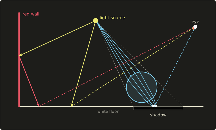
- Direct light (直接光): lamp → floor → eye. This is what chapter 10 computed.
- Shadow (影): the ball blocks the lamp, so part of the floor gets no direct light (chapter 11).
- Interreflection (相互反射): lamp → red wall → floor → eye. The floor receives light that the wall has already colored, so it turns slightly red near the wall. This tint is called color bleeding (カラーブリーディング).
- Caustic (コースティクス): lamp → glass ball → floor → eye. The ball bends the light and focuses it into a bright spot, right in the middle of its own shadow.
A local illumination (局所照明) model computes the color of a point from the point itself, its normal, its material and the light sources, as if nothing else existed in the scene.
The Phong model of chapter 10 is local: it never asks what else is around.
A global illumination (大域照明) model also accounts for the light that arrives via other surfaces: reflections, refractions, interreflection, caustics, and shadows as a matter of course.
Global illumination is what makes an image photorealistic (写実的), and it is expensive, because every point now depends on every other point.
Local models fake the missing light with the ambient term (環境光項) of chapter 10, a constant that lifts the dark parts.
It's a single number for the whole scene, so it can't make the floor red near a red wall or dark in a corner.
Naming light paths
A compact way to say which paths a method handles is Heckbert's light path notation (Paul Heckbert, 1990).
A path is written as a string of letters: L for the light, E for the eye, D for a diffuse bounce and S for a specular (mirror or glass) bounce, with the usual pattern symbols: * for "any number", + for "one or more", ? for "zero or one", | for "or".
- Direct light on a matte floor:
LDE. Color bleeding:LDDE. A caustic on the floor:LSDE(more generallyLS+DE). - Everything that can happen:
L(D|S)*E.
We'll use this notation to compare the methods of this chapter in section 12.12.
12.2 Measuring light
Chapter 10 multiplied colors without ever asking about units.
To talk about bouncing light we need a little radiometry (放射測定), the measurement of light energy.
Light from chapter 3 is an electromagnetic wave carrying energy; here we only count how much energy flows where.
Solid angle (立体角) is the 3D version of an angle: the area a cone of directions cuts out of a sphere of radius 1.
Its unit is the steradian (ステラジアン, sr).
The whole sphere is sr, a hemisphere sr.
A small patch of area seen from distance , facing us, covers about steradians.
The four quantities worth knowing:
| Quantity | Symbol | Unit | Meaning |
|---|---|---|---|
| radiant flux (放射束) | W | total light power, e.g. of a lamp | |
| radiant intensity (放射強度) | W/sr | power per solid angle, how bright a point light is in one direction | |
| irradiance (放射照度) | W/m² | power arriving per area of a surface, from all directions | |
| radiance (放射輝度) | W/(m²·sr) | power per area per solid angle: light traveling along one ray |
Radiance is the quantity a camera pixel or an eye measures, and the one a renderer computes for every pixel.
It has a property that makes ray tracing possible: in empty space radiance stays constant along a ray.
A wall twice as far away covers a quarter of the solid angle but each point sends the same radiance, which is why a white wall looks equally bright from near and far.
The photometric quantities of chapter 3 are the same ideas weighted by the eye's sensitivity: luminance (輝度, cd/m²) from chapter 3 is the photometric partner of radiance, illuminance (照度, lux) the partner of irradiance.
Worked example: irradiance
A point light. A point light with radiant intensity W/sr hangs m from a point on the floor, and the light arrives at from the floor's normal.
The irradiance falls with the square of the distance (the attenuation of chapter 10) and with the cosine of the angle (Lambert's cosine law, chapter 10):
A uniform sky. Now light comes from every direction of the hemisphere with the same radiance .
Each direction contributes per steradian, so
is the hemisphere above the point, a tiny piece of solid angle, and the integral sign just means "add up over all directions".
The result is and not (the hemisphere's size), because directions near the horizon are weighted by a cosine close to 0.
For a sky with W/(m²·sr) the irradiance is W/m².
This factor shows up again in a moment.
12.3 The BRDF
How a surface turns incoming light into outgoing light is described by its BRDF (双方向反射率分布関数, bidirectional reflectance distribution function), written .
For light arriving from direction it tells how much radiance leaves in direction , per unit of irradiance:
"Bidirectional" because it depends on two directions, in and out.
The BRDF is the physical version of the "material" of chapter 10.
Drawn as a lobe (the length of each arrow is the reflected amount in that direction), three typical shapes look like this:
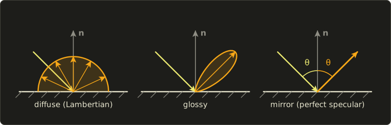
- Diffuse (拡散反射): the reflected radiance is the same in every direction, so the surface looks equally bright from anywhere (paper, matte paint, plaster). The ideal case is the Lambertian surface (完全拡散反射面, ランバート面).
- Glossy (光沢): most light goes near the mirror direction, spread into a lobe (plastic, varnished wood, brushed metal). Chapter 10's specular highlight is a glossy lobe.
- Mirror, perfect specular (鏡面反射): all light leaves in exactly one direction, the reflection of the incoming direction (a mirror, a calm lake, polished chrome).
Real materials are mixtures, e.g. a diffuse base under a glossy varnish.
Properties of a physical BRDF
- Non-negative: . A surface can't reflect negative light.
- Reciprocity (相反性, Helmholtz reciprocity): . Swapping light and eye gives the same value. This is what allows tracing rays backwards from the eye, as ray tracing does.
- Energy conservation (エネルギー保存): a surface can't reflect more than it receives. For every incoming direction, .
The fraction of the incoming light that is reflected in total is the albedo (アルベド, 反射率) , a number between 0 and 1.
Fresh snow has an albedo of about 0.9, asphalt about 0.1.
Worked example: the Lambertian BRDF
A Lambertian surface has the same BRDF for all directions: a constant .
Energy conservation tells us what the constant must be.
The reflected fraction is (the same as for the sky), and it must equal the albedo :
A white plaster wall with has per steradian.
Under the point light of section 12.2 ( W/m²), the radiance it sends in every direction is
That is why physically based renderers divide the diffuse color by , and why the light intensities in their scenes look " times too big" when you come from the Phong model.
You'll see the same factor in the OpenGL series, chapter 24.
The Phong model of chapter 10 doesn't conserve energy in general: with a large it can send out more light than arrives.
Microfacets, briefly
A rough surface is, under a microscope, a landscape of tiny flat mirrors, microfacets (マイクロファセット).
Light that reaches the eye was mirrored by those facets whose normal happens to lie halfway between the light and the eye, the half vector of Blinn–Phong.
The Cook–Torrance model (Robert Cook and Kenneth Torrance, 1982) builds a BRDF from three factors: how many facets face (the distribution D), how many of them are neither shadowed nor hidden by other facets (the geometry term G), and how much one facet reflects at this angle (the Fresnel term F):
A smooth surface has a narrow D (a sharp highlight), a rough one a wide D (a blurry one).
This is the basis of today's physically based rendering (PBR, 物理ベースレンダリング); Part 2 covers it fully, and you'll implement it in OpenGL chapter 24.
Light that goes through a surface is described the same way by a BTDF (bidirectional transmittance distribution function); BRDF and BTDF together form the BSDF (bidirectional scattering distribution function).
Exam points
- BRDF = outgoing radiance per incoming irradiance, depends on two directions, unit 1/sr, can be larger than 1 (a sharp mirror lobe).
- Reciprocity: in and out can be swapped. Energy conservation: total reflection ≤ incoming.
- Lambertian BRDF = ; the reflected radiance is the same from every viewing direction (view independent).
- Microfacet model (Cook–Torrance): D × F × G.
12.4 The Fresnel effect
Look at a window or a lake: head-on you see through it, at a grazing angle it becomes a mirror.
How much light a smooth boundary between two materials reflects depends on the angle; this is the Fresnel effect (フレネル効果), described by the Fresnel equations of optics.
The materials are characterized by their refractive index (屈折率) : 1 for vacuum (air is 1.0003, close enough to 1), about 1.33 for water and about 1.5 for glass.
Head-on (angle of incidence 0°) the reflectance of a boundary from to is
For air to glass: .
For air to water: .
So glass reflects 4% of the light head-on, water 2%.
The rest goes into the material (refraction, next section).
The exact equations treat the two polarizations of light separately and are a bit long.
Schlick's approximation (Christophe Schlick, 1994) is what nearly every renderer uses:
is the angle between the incoming ray and the normal.
At 0° it gives , at 90° (grazing) it gives exactly 1: every surface becomes a perfect mirror at grazing angles.
Worked example: glass and water
At : , so , and
The whole table, with the exact Fresnel value for glass (unpolarized light) to show how good the approximation is:
| θ | cos θ | glass, Schlick | glass, exact | water, Schlick | |
|---|---|---|---|---|---|
| 0° | 1 | 0 | 0.040 | 0.040 | 0.020 |
| 30° | 0.866 | 0.00004 | 0.040 | 0.042 | 0.020 |
| 45° | 0.707 | 0.0022 | 0.042 | 0.050 | 0.022 |
| 60° | 0.5 | 0.0313 | 0.070 | 0.089 | 0.051 |
| 75° | 0.259 | 0.2237 | 0.255 | 0.253 | 0.239 |
| 85° | 0.087 | 0.6339 | 0.649 | 0.613 | 0.641 |
| 90° | 0 | 1 | 1 | 1 | 1 |
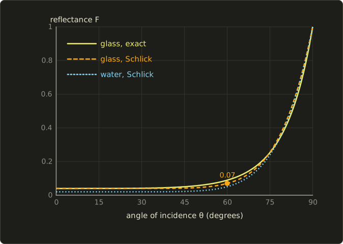
The reflectance hardly changes until about 60°, then climbs steeply.
Schlick is off by a few hundredths in places, which is invisible in practice, and it costs one subtraction and a few multiplications.
In practice
- Water and glass: a lake reflects the far shore (grazing angles) but lets you see the bottom at your feet (steep angles). Without Fresnel, rendered water looks like plastic.
- Every material has Fresnel: even matte objects get a bright rim at grazing angles. PBR materials store ; for non-metals it is about 0.04, which is why many engines use 0.04 as the default.
- Metals reflect a lot head-on, and their depends on the wavelength: the yellow of gold and the orange of copper are their Fresnel color.
- The Fresnel weight decides the split between reflection and refraction: a fraction F of the light is reflected and is transmitted. Ray tracers use it exactly like that (section 12.8).
12.5 Refraction
The light that isn't reflected enters the material and changes direction: refraction (屈折).
The cause is that light travels more slowly in the denser material (by the factor ).
Snell's law (スネルの法則) relates the angles to the normal on both sides:
Going into a denser material () the ray bends towards the normal; coming out it bends away from it.
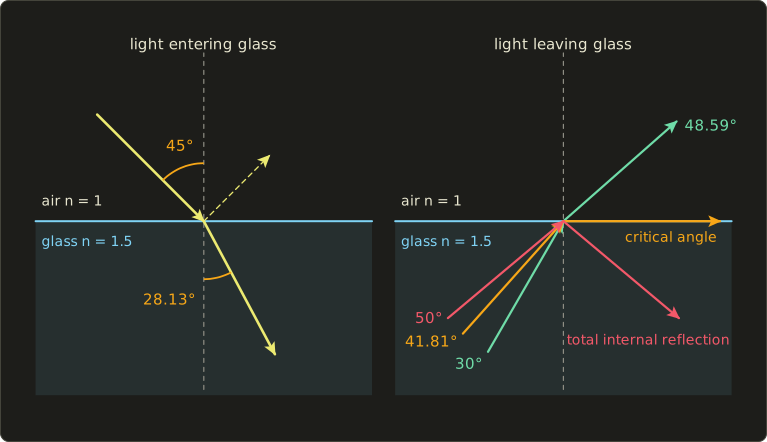
Worked example: Snell's law
Air to glass at :
Air to water at 45°: , so .
Water bends light less than glass because its index is closer to 1.
Total internal reflection
Now go the other way, from glass () into air ().
At 30° inside the glass: , so the ray leaves at 48.59°.
At 50°: .
A sine can't be larger than 1, so there is no refracted ray at all: all the light is reflected back into the glass.
This is total internal reflection (全反射).
It starts at the critical angle (臨界角), where the refracted ray would just graze the surface ():
Total internal reflection only happens when light goes from the denser to the less dense material.
In practice
- Optical fibers keep light inside by total internal reflection, and the sparkle of a cut diamond comes from its very high index (about 2.42, so a critical angle of only about 24°): light bounces around inside many times before it escapes.
- Snell's window: a diver looking up sees the whole sky squeezed into a circle of half-angle 48.75° (97.5° across); outside it the water surface is a mirror.
- Dispersion (分散): the index depends slightly on the wavelength (blue is bent more than red), which is how a prism splits white light into a spectrum and how rainbows form. A renderer needs spectral rendering (several wavelengths instead of RGB) to show it.
- In a ray tracer, the refracted direction is computed in vector form. With unit incoming direction , unit normal facing the incoming ray, and :
If we have total internal reflection.
is , so this is Snell's law written with vectors.
GLSL, Slang and HLSL have it built in as refract(d, n, eta), which returns a zero vector when .
12.6 Light inside materials and in the air
Everything so far happened exactly at the surface.
Many materials let light in and scatter it around before it comes out again.
Translucency and subsurface scattering
Shine a flashlight through your fingers and they glow red.
In skin, marble, wax, milk, jade or leaves, light enters the material, is scattered many times inside, and leaves at a different point, often several millimeters away.
This is subsurface scattering (表面下散乱), and materials like this are translucent (半透明).
A BRDF assumes light leaves where it arrived, so it can't describe this; the generalization is the BSSRDF (bidirectional scattering-surface reflectance distribution function), which also depends on the entry and exit points.
Without subsurface scattering skin looks like painted plastic or wax figures look like stone: the soft light bleeding into shadows and the reddish glow at thin parts (ears, nostrils) are missing.
Film renderers simulate it; games approximate it, e.g. by blurring the lighting on skin in screen space.
Participating media
Fog, smoke, clouds, murky water and even clear air are participating media (関与媒質): the space between surfaces itself takes part in the light transport.
Along a ray, light can be absorbed (吸収, turned into heat), scattered out of the ray, or scattered into it from elsewhere (which makes fog glow around lamps and creates visible light shafts).
The simplest piece is the Beer–Lambert law (ランベルト・ベールの法則): through a uniform medium the fraction of light that gets through a distance is
where (per meter) says how dense the medium is.
Worked example: fog with per meter lets of the light through over 10 m, and only over 30 m.
Classic "exponential fog" in games is exactly this: pixel color .
Why the sky is blue
Air molecules are far smaller than the wavelength of light, and for such tiny particles the scattering strength grows as : Rayleigh scattering (レイリー散乱).
Blue light at 450 nm is therefore scattered
times more strongly than red light at 700 nm.
Sunlight crossing the atmosphere loses its blue to all sides, and that scattered blue reaches us from every direction of the sky.
At sunset the light travels a much longer path through the air, most of the blue is scattered away before it reaches us, and the sun and clouds turn orange and red.
Particles comparable to or larger than the wavelength (water droplets, dust, smoke) scatter all wavelengths about equally and mostly forwards: Mie scattering (ミー散乱).
That's why clouds are white, haze is gray-white, and there is a bright glow around the sun on a hazy day.
Sky models in games and film are built on these two kinds of scattering; volume rendering is covered in Part 2.
Caustics
A caustic (コースティクス) is light focused by curved mirrors or lenses onto a diffuse surface: the bright net of lines at the bottom of a swimming pool, the bright spot under a glass of water, the heart-shaped curve inside a coffee cup in the sun.
In path notation it is LS+DE: one or more specular bounces, then a diffuse surface, then the eye.
Caustics are among the hardest effects to render, as we'll see: they need a method that follows light from the lamp.
12.7 The rendering equation
All of this fits into a single equation, the rendering equation (レンダリング方程式), introduced in 1986 by James Kajiya (and in the same year, independently, by David Immel and colleagues).
In the form usually written today:
Read it from left to right:
- : the radiance leaving point in direction (towards the eye). This is what a pixel shows.
- : the radiance the point emits itself (nonzero only for light sources).
- The integral: add up, over all incoming directions of the hemisphere, the incoming radiance , weighted by the BRDF and by the cosine of the angle to the normal (Lambert's cosine law).
The catch is .
The light arriving at from direction is the light leaving whatever surface point we see in that direction: .
The unknown appears on both sides; every point depends on every other point.
That is global illumination in one line.
Every method is an approximation
| Method | What it does with the integral |
|---|---|
| local illumination (chapter 10) | keeps only the point lights: the integral becomes a sum over the lamps; everything else is the ambient constant |
| Whitted ray tracing | point lights, plus exactly one direction for a mirror and one for a refraction, followed recursively |
| distributed ray tracing / path tracing | estimates the integral with random sample directions (Monte Carlo) |
| radiosity | assumes every surface is Lambertian and solves for the light of small patches |
| photon mapping | sends light from the lamps first, stores it, then estimates the integral from the stored photons |
Worked example: why the bounces matter
Imagine a closed room whose walls all have albedo , and suppose the lamps give every wall the radiance by direct light.
After one bounce each wall also receives a fraction of that, after two bounces , and so on.
The total is a geometric series:
For white walls with the room is times brighter than direct light alone suggests; for it is twice as bright.
In a white room, most of the light you see has bounced several times, which is why a local model with a guessed ambient term looks so flat.
12.8 Ray tracing
Chapter 6 drew triangles by projecting them onto the screen.
Ray tracing (レイトレーシング法) goes the other way round: for every pixel it shoots a ray from the eye through the pixel into the scene and asks what that ray hits.
Because it follows light against the direction light actually travels, tracing from the eye is often called backward tracing (逆方向), and tracing from the lights, as photon mapping does in section 12.12, forward tracing (順方向); be aware that some books use the two words the other way round.
Following one ray to its first hit is ray casting (レイキャスティング法), which chapter 10 used for hidden surface removal.
Ray tracing, in the form Turner Whitted published in 1980 ("An Improved Illumination Model for Shaded Display"), continues recursively at the hit point:
- The primary ray (一次レイ, eye ray) goes from the eye through the pixel to the first hit.
- From the hit, a shadow ray (シャドウレイ) goes to each light. If something blocks it, that light doesn't count (chapter 11).
- If the surface is a mirror, a reflection ray (反射レイ) is traced in the mirror direction (Linear Algebra chapter 4).
- If it is transparent, a refraction ray (屈折レイ, transmission ray) is traced in the Snell direction of section 12.5.
- The reflection and refraction rays hit other surfaces, which spawn their own shadow, reflection and refraction rays, and so on.
All the rays spawned by one primary ray form a ray tree (レイツリー).
The pixel's color is collected from the leaves upwards: each node adds its local lighting and the weighted colors of its children.
Because the tree could grow forever between two mirrors, the recursion stops at a maximum depth (typically 5 to 10) or when the weight of a branch becomes negligible.
In pseudo-code:
color trace(ray, depth):
    hit = nearest intersection of ray with the scene
    if there is no hit: return background color
    color = local lighting at hit            (one shadow ray per light)
    if depth < maxDepth:
        if hit is reflective:  color += kr * trace(reflection ray, depth + 1)
        if hit is transparent: color += kt * trace(refraction ray, depth + 1)
    return color
For glass, and are the Fresnel weights and of section 12.4.
Whitted's ray tracer gives sharp reflections, refraction and exact hard shadows, things a rasterizer can only fake.
What it can't do is just as important (and worth knowing for the exam):
- No diffuse interreflection: the light that bounces off a matte wall is never followed, so there is no color bleeding and the ambient term is still a constant.
- No soft shadows: point lights only, one shadow ray each.
- No glossy reflection: a reflection ray goes in exactly one direction, so reflections are always perfectly sharp.
- No caustics: shadow rays go straight to the lamp, so light focused by glass never arrives (the shadow of a glass ball is completely black).
Ray–sphere intersection
The heart of a ray tracer is the intersection test.
A ray starts at and goes in the unit direction ; its points are for , and is the distance along the ray.
A sphere with center and radius is the set of points at distance from the center: .
Put the ray into the sphere equation, with :
(the term has the factor because is a unit vector).
That's a quadratic equation.
With and the school formula simplifies to
The sign of the discriminant tells the story: negative, the ray misses; zero, it just touches; positive, it enters at the smaller and leaves at the larger one.
We want the smallest that is positive (a negative lies behind the ray's start).
Worked example: one ray through a glass ball
The ray starts at the eye and goes in the direction , a unit vector because .
The glass ball has center and radius .
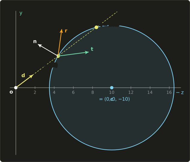
Intersection. .
Both are positive, so the ray enters at and would leave at .
The hit point is .
Normal. The normal of a sphere points from the center to the hit point; dividing by makes it a unit vector:
(Check: .)
Angle of incidence.
That's exactly , so and : the ray hits the ball at a fairly grazing angle.
Fresnel. With Schlick and :
So 12.5% of the pixel's color comes from the reflection ray and 87.5% from the refraction ray.
Reflection ray. , so
Refraction ray. Air to glass, :
Check with Snell: , so and , as it should be.
The ray tracer now calls trace for and and mixes the results as .
Here are the same steps in C++ with the linalg.hh header of the Linear Algebra series (reflect is the function from Linear Algebra chapter 4):
#include <cmath>
#include <cstdio>
#include "linalg.hh"

// Distance t to the nearest hit of the ray o + t d (d normalized) with a sphere, or -1 for a miss.
float hitSphere(Vec3 o, Vec3 d, Vec3 c, float r) {
  Vec3 m = o - c;
  float b = dot(m, d);
  float cc = dot(m, m) - r * r;
  float disc = b * b - cc;
  if (disc < 0.0f) return -1.0f;  // the ray misses the sphere
  float s = std::sqrt(disc);
  float t = -b - s;               // the nearer root first
  if (t < 1e-4f) t = -b + s;      // we start inside the sphere
  return t < 1e-4f ? -1.0f : t;   // the whole sphere is behind us
}

Vec3 reflect(Vec3 d, Vec3 n) { return d - 2.0f * dot(d, n) * n; }

// eta = n1 / n2. Returns false on total internal reflection.
bool refract(Vec3 d, Vec3 n, float eta, Vec3 *t) {
  float cosI = -dot(d, n);
  float k = 1.0f - eta * eta * (1.0f - cosI * cosI);
  if (k < 0.0f) return false;
  *t = eta * d + (eta * cosI - std::sqrt(k)) * n;
  return true;
}

float schlick(float cosTheta, float f0) {
  float m = 1.0f - cosTheta;
  return f0 + (1.0f - f0) * m * m * m * m * m;
}

int main() {
  Vec3 o{0, 0, 0}, d{0, 0.6f, -0.8f}, c{0, 0, -10};
  float r = 6.5f;
  float t = hitSphere(o, d, c, r);
  Vec3 p = o + t * d;
  Vec3 n = (p - c) / r;
  float cosI = -dot(d, n);
  Vec3 refl = reflect(d, n), refr;
  refract(d, n, 1.0f / 1.5f, &refr);
  printf("t = %.4f, p = (%.4f, %.4f, %.4f)\n", t, p.x, p.y, p.z);
  printf("n = (%.4f, %.4f, %.4f), cos = %.4f\n", n.x, n.y, n.z, cosI);
  printf("Fresnel (Schlick, glass) = %.4f\n", schlick(cosI, 0.04f));
  printf("reflected = (%.4f, %.4f, %.4f)\n", refl.x, refl.y, refl.z);
  printf("refracted = (%.4f, %.4f, %.4f)\n", refr.x, refr.y, refr.z);

  // inside the glass, 50 degrees from the normal: beyond the critical angle
  float a = 50.0f * 3.14159265f / 180.0f;
  Vec3 inside{std::sin(a), std::cos(a), 0};  // travelling up towards the glass-air surface
  Vec3 facing{0, -1, 0};                     // the normal on the side the ray comes from
  Vec3 out;
  bool ok = refract(inside, facing, 1.5f, &out);
  printf("50 degrees inside the glass: %s\n", ok ? "refracts" : "total internal reflection");
  return 0;
}
t = 5.5000, p = (0.0000, 3.3000, -4.4000)
n = (0.0000, 0.5077, 0.8615), cos = 0.3846
Fresnel (Schlick, glass) = 0.1247
reflected = (0.0000, 0.9905, -0.1373)
refracted = (0.0000, 0.1300, -0.9915)
50 degrees inside the glass: total internal reflection
Planes and triangles, briefly
As in section 10.5, a plane through point with normal is hit at
If the ray is parallel to the plane.
Example: the floor (, ) and a ray from the origin in direction : .
A triangle is a plane hit followed by an inside test, usually with barycentric coordinates like the edge functions of chapter 6; the Möller–Trumbore algorithm does both at once and is what most ray tracers use for triangle meshes.
In a shader: Fresnel-weighted glass
A real-time renderer can get the look of a glass object cheaply by combining the environment mapping of chapter 11 with the Fresnel weight: look up the sky in the reflection and refraction directions and mix them with .
(It refracts only once and ignores the back of the object, a common approximation.)
TextureCube<float4> sky;
SamplerState skySampler;

float schlick(float cosTheta, float f0) {
  float m = saturate(1.0 - cosTheta);
  return f0 + (1.0 - f0) * m * m * m * m * m;
}

// d: unit direction from the eye to the surface, n: unit normal facing the eye
float3 glassColor(float3 d, float3 n) {
  const float eta = 1.0 / 1.5;  // air -> glass
  float f0 = (1.0 - 1.5) / (1.0 + 1.5);
  f0 = f0 * f0;                 // 0.04
  float F = schlick(-dot(d, n), f0);
  float3 reflected = sky.Sample(skySampler, reflect(d, n)).rgb;
  float3 refracted = sky.Sample(skySampler, refract(d, n, eta)).rgb;
  return lerp(refracted, reflected, F);
}layout(set = 0, binding = 1) uniform samplerCube sky;
float schlick(float cosTheta, float f0) {
float m = clamp(1.0 - cosTheta, 0.0, 1.0);
return f0 + (1.0 - f0) * m * m * m * m * m;
}
// d: unit direction from the eye to the surface, n: unit normal facing the eye
vec3 glassColor(vec3 d, vec3 n) {
const float eta = 1.0 / 1.5; // air -> glass
float f0 = (1.0 - 1.5) / (1.0 + 1.5);
f0 = f0 * f0; // 0.04
float F = schlick(-dot(d, n), f0);
vec3 reflected = texture(sky, reflect(d, n)).rgb;
vec3 refracted = texture(sky, refract(d, n, eta)).rgb;
return mix(refracted, reflected, F);
}TextureCube<float4> sky;
SamplerState skySampler;
float schlick(float cosTheta, float f0) {
float m = saturate(1.0 - cosTheta);
return f0 + (1.0 - f0) * m * m * m * m * m;
}
// d: unit direction from the eye to the surface, n: unit normal facing the eye
float3 glassColor(float3 d, float3 n) {
const float eta = 1.0 / 1.5; // air -> glass
float f0 = (1.0 - 1.5) / (1.0 + 1.5);
f0 = f0 * f0; // 0.04
float F = schlick(-dot(d, n), f0);
float3 reflected = sky.Sample(skySampler, reflect(d, n)).rgb;
float3 refracted = sky.Sample(skySampler, refract(d, n, eta)).rgb;
return lerp(refracted, reflected, F);
}You'll build a full sky cube map and reflections yourself in the OpenGL series, chapter 18, and a ray-based renderer in a fragment shader in the GLSL series, chapter 14.
12.9 Making ray tracing fast
A naive ray tracer tests every ray against every object.
A Full HD image has pixels; with a scene of one million triangles that's about triangle tests for the primary rays alone, before a single shadow or reflection ray.
Almost all of these tests are wasted, because a ray only passes near a tiny part of the scene.
Acceleration structures (高速化データ構造) skip whole groups of objects with one cheap test.
Bounding volumes
A bounding volume (バウンディングボリューム) is a simple shape that encloses a complicated object: a sphere or an axis-aligned box (AABB).
If the ray misses the box, it misses everything inside, and testing a ray against a box takes only a few multiplications (the "slab test": clip the ray's range against the three pairs of parallel planes; the ray hits the box if the range doesn't become empty).
Bounding volume hierarchy (BVH)
Put bounding volumes inside bounding volumes and you get a tree, the BVH (階層バウンディングボリューム).
The root box contains the whole scene, its children contain halves of it, and so on down to a few triangles per leaf:
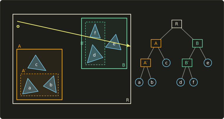
The ray in the picture misses box A, so the whole left subtree (A′, a, b and c) is skipped after a single box test.
It hits B, so B′ and e are tested, and then d and f inside B′.
For a balanced tree over triangles, the depth is about : for a million triangles, .
A ray then needs a few dozen box tests and a handful of triangle tests instead of a million.
Spatial subdivision
Instead of grouping objects, we can divide space:
- Uniform grid (均一格子): cut the scene's box into equal cells; each cell lists the objects overlapping it. The ray walks from cell to cell along its path (like a 3D line-drawing algorithm from chapter 6) and stops at the first cell with a hit. Simple, but wasteful when objects are clustered.
- Octree (八分木): cut a cell into 8 equal children only where there are many objects. Adapts to the scene.
- kd-tree (kd木): cut a cell in two with a plane perpendicular to one axis, placed wherever it best separates the objects; the axis alternates or is chosen per node.
| Structure | Divides | Strength | Weakness |
|---|---|---|---|
| BVH | objects into nested boxes | each object in exactly one leaf; fast to rebuild for moving objects | boxes can overlap |
| uniform grid | space into equal cells | very simple, fast to build | bad for scenes with crowded and empty areas |
| octree | space into 8 children where needed | adapts to the density | fixed split positions |
| kd-tree | space by axis-aligned planes at any position | very fast traversal for static scenes | objects may be in several cells; slow to rebuild |
The same structures speed up collision detection in games and physics (chapter 14).
Modern GPUs have ray tracing hardware (since 2018), and the ray tracing APIs of Vulkan and DirectX 12 build BVH-like acceleration structures for you: a bottom level per mesh and a top level over the instances.
12.10 Distributed ray tracing and path tracing
Whitted's rays go in exactly one direction each, so everything is perfectly sharp.
In 1984 Robert Cook, Thomas Porter and Loren Carpenter showed in "Distributed ray tracing" that the missing effects appear when rays are spread out over a range and averaged.
This is distributed ray tracing (分散レイトレーシング, also called stochastic ray tracing):
| Spread the rays over | Effect |
|---|---|
| the pixel area | anti-aliasing (chapter 2's supersampling) |
| the area of the light | soft shadows with penumbrae |
| a cone around the mirror direction | glossy (blurry) reflections |
| the lens area | depth of field (chapter 2's thin lens) |
| the time the shutter is open | motion blur |
Each of these is an integral (over an area, a cone, an interval) and the average of random samples estimates it.
That idea has a name.
Monte Carlo integration
To estimate an integral , pick random points with probability density and average:
This is Monte Carlo integration (モンテカルロ法).
On average it gives exactly the right answer (it is unbiased), but each estimate is off by random noise, and the noise shrinks only with the square root of the number of samples:
Worked example. Estimate , which we know is .
Pick directions uniformly on the hemisphere, , so each sample contributes .
Four random directions with give
10% too high.
How large is the noise?
For uniformly distributed directions on a hemisphere, is uniformly distributed between 0 and 1, whose standard deviation is ; one sample therefore has an error of , more than half of .
With samples:
| N | expected error | relative to π |
|---|---|---|
| 1 | 1.814 | 58% |
| 16 | 0.453 | 14% |
| 256 | 0.113 | 3.6% |
Every factor 4 in samples halves the error, every factor 16 divides it by 4, and going from 10% noise to 1% costs 100 times the work.
A quick experiment (10,000 estimates for each ) measures RMS errors of 1.835, 0.460 and 0.113, matching the table.
Importance sampling (重点的サンプリング) reduces the noise without more samples: choose similar in shape to .
Here, picking directions with density (more directions near the normal) makes every sample : the exact answer with zero noise.
In a real scene also contains the unknown incoming light, so the noise never vanishes, but sampling proportional to the BRDF and the cosine, and sending extra rays towards the lights, removes most of it.
Path tracing
Path tracing (パストレーシング法), introduced by Kajiya together with the rendering equation in 1986, solves that equation with Monte Carlo.
Instead of a tree of rays, each sample is a single path: from the eye to a surface, then in one randomly chosen direction to the next surface, and so on, until it reaches a light or is stopped.
Every pixel averages many such paths (the samples per pixel, spp).
color radiance(ray):
    result = 0, weight = 1
    repeat:
        hit = nearest intersection of ray with the scene
        if there is no hit: return result
        result += weight * (light emitted at hit)
        result += weight * (direct light from one random point on a lamp)   (shadow ray)
        choose a new direction w with probability p(w)
        weight *= brdf * cos / p(w)
        (Russian roulette) stop with probability 1 - q, otherwise weight /= q
        ray = new ray from hit in direction w
Because diffuse surfaces scatter in random directions, a path tracer gets everything: color bleeding, soft shadows from area lights, glossy reflections, and (slowly) caustics.
The price is noise.
Here is a small path tracer (a NumPy script, about 100 lines) rendering a box with a red and a green wall, a white ball and a glass ball under a square ceiling lamp, with 1, 16 and 256 samples per pixel; the error is measured against a reference image with 2048 samples:
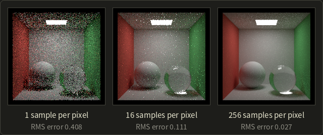
The measured errors drop by factors of 3.7 and 4.1 for each 16× more samples, close to the that Monte Carlo predicts.
The bright speckles that stay longest sit around the glass ball: they are caustic paths (LSDE), which a path from the eye finds only by luck.
Next to it, the same scene rendered the Whitted way, with one point light at the position of the lamp:
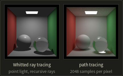
The Whitted image has sharp black shadows, a black ceiling (no lamp shines on it) and no colored light on the white surfaces.
The path-traced image has soft shadows, a ceiling lit by light bounced off the floor and walls, red and green bleeding onto the white surfaces, and the caustic under the glass ball.
Russian roulette (ロシアンルーレット) ends paths without bias.
After a few bounces a path continues with probability and stops otherwise; a surviving path divides its weight by .
On average nothing changes: a contribution of 0.5 with becomes in 70% of the cases and 0 in the rest, and .
But most dim paths stop early, which saves a lot of time.
In practice
Film production moved to path tracing over the last decades; renderers such as Arnold, RenderMan and Blender's Cycles are path tracers.
Bidirectional path tracing (双方向パストレーシング) builds paths from the eye and from the lights and connects them, which finds caustics much faster.
Games use hardware ray tracing for reflections, shadows and some global illumination with only one or two samples per pixel and then remove the noise with a denoiser (a filter that smooths the noise while keeping edges, often a neural network).
Part 2 goes deeper into Monte Carlo rendering.
12.11 Radiosity
Path tracing computes the light for one viewpoint, pixel by pixel.
Radiosity (ラジオシティ法) takes a completely different approach, borrowed from heat transfer engineering and brought to graphics in 1984 by Cindy Goral, Kenneth Torrance, Donald Greenberg and Bennett Battaile at Cornell University ("Modeling the interaction of light between diffuse surfaces").
Their test scene was a cube with a red and a blue wall, and the point of the paper was exactly the color bleeding that no earlier method could produce.
The idea:
- Assume every surface is Lambertian (perfectly diffuse). Then the light leaving a point is the same in every direction, and one number per point (per color channel) describes it.
- Divide all surfaces into small patches (パッチ) and assume the light is constant over each patch.
- Write the light balance between all patches as a system of linear equations and solve it.
The light leaving patch per area is its radiosity (radiant exitance, 放射発散度, W/m²).
It is what the patch emits plus what it reflects of the light from all other patches:
is the emitted light (nonzero for lamps), the albedo and the form factor (形態係数).
For a Lambertian patch the radiance is , which is what the screen shows.
Form factors
is the fraction of the light leaving patch that arrives at patch .
It depends only on the geometry: the sizes, distance and orientations of the two patches, and whether something blocks the view between them.
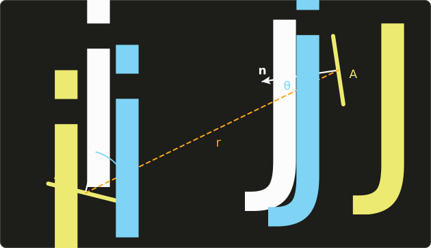
is 1 where the two points see each other and 0 where something is in between.
The integrals average over all pairs of points; for patches that are small compared to their distance, the integrand hardly changes and
Worked examples: two small patches facing each other directly () 1 m apart, with m² (10 cm × 10 cm): .
Tilt both by 60° and move them to 2 m: , sixteen times less (a quarter from the cosines, a quarter from the distance).
Properties worth knowing:
- Reciprocity (相反性): . A large patch sends a smaller fraction of its light to a small patch than the other way round.
- Summation: in a closed scene ; all the light leaving a patch lands somewhere.
- for a flat patch (it can't see itself), and .
- Form factors don't depend on materials or lights, so they are computed once for a static scene.
Computing them is the expensive part.
The Nusselt analog gives a picture: project patch onto a unit hemisphere around patch , then straight down onto the base disk; the form factor is the projected area divided by the disk's area .
The hemicube method (Michael Cohen and Donald Greenberg, 1985) puts half a cube around each patch, renders the scene onto its faces with a Z-buffer, and adds up precomputed weights of the pixels each patch covers, which also handles occlusion for free.
Worked example: three patches and color bleeding
A lamp, a white floor and a red wall, all of the same area (so by reciprocity).
The form factors are , and ; the rest of the light leaves the scene.
The lamp emits in every channel and reflects nothing; the floor has , the wall .
The lamp's radiosity is just .
For the red channel, floor (W) and wall (R) give
Substitute the second into the first: , so
For the green (and blue) channel the wall only reflects 0.1:
With direct light only, the floor would be , a neutral gray.
With the interreflection it is : its red channel is 9.4% stronger than green and blue.
The white floor has turned pinkish because of the red wall: color bleeding, computed.
Solving the system: Jacobi and Gauss–Seidel
Real scenes have thousands of patches, too many to substitute by hand.
The equations have the form ( is the diagonal matrix of albedos), i.e. the linear system .
Because every and every row of adds up to at most 1, simple iteration converges:
- Jacobi iteration: start with and compute all new values from the old ones: . Iteration contains exactly the light paths with up to bounces.
- Gauss–Seidel iteration: the same, but each new value is used immediately for the following patches in the same sweep. Here it needs about half as many sweeps.
The red channel of our example ( stays 10):
| iteration | Jacobi | Jacobi | Gauss–Seidel | Gauss–Seidel |
|---|---|---|---|---|
| 0 | 0 | 0 | 0 | 0 |
| 1 | 3.2 | 1.6 | 3.2 | 2.112 |
| 2 | 3.456 | 2.112 | 3.5379 | 2.1661 |
| 3 | 3.5379 | 2.1530 | 3.5466 | 2.1675 |
| 4 | 3.5445 | 2.1661 | 3.5468 | 2.1675 |
| exact | 3.5468 | 2.1675 | 3.5468 | 2.1675 |
In the first Gauss–Seidel sweep the wall already uses the new floor value 3.2: .
Progressive refinement (漸進的改良法; Cohen, Chen, Wallace and Greenberg, 1988) turns the computation around: instead of every patch gathering light from all others, the patch with the most not-yet-distributed light shoots it to all others, then the next brightest, and so on.
A useful image appears after the first few steps (the lamps have shot their light), and it improves continuously, which made radiosity practical for interactive design.
Rendering the result
Once the radiosities are known they belong to the scene, not to a camera.
Radiosity is view independent (視点非依存): you can walk through the scene and render each frame with ordinary rasterization, using the patch values as vertex colors.
Here is the empty box from the path-tracing example, solved with 8 × 8 patches per wall (320 patches, form factors computed numerically):
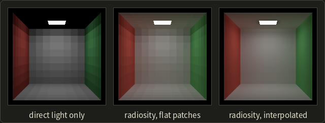
With direct light only (one Jacobi step) the ceiling is black.
The full solution lights it with bounced light and tints the white surfaces near the colored walls.
Drawn with one color per patch the patches show as squares; interpolating the values between patch centers (like Gouraud shading in chapter 10) makes it smooth.
Limits
- Diffuse only: no mirrors, no glossy highlights, no refraction, so no caustics either. Radiosity's strength (view independence) comes from exactly this assumption.
- Meshing: sharp shadow edges need small patches, and the number of form factors grows with the square of the number of patches.
- In practice it was often combined with ray tracing in two-pass methods: radiosity for the diffuse light, then a ray-tracing pass from the eye for specular effects.
Precomputed diffuse lighting stored in textures (light maps, ライトマップ, chapter 11) is the same idea in today's games: compute the bounced light offline once, then just look it up.
12.12 Photon mapping and real-time global illumination
Photon mapping
Caustics are hard for anything that starts at the eye: the path must hit the small lamp exactly after passing through the glass.
Photon mapping (フォトンマッピング法), developed by Henrik Wann Jensen (first published with Niels Jørgen Christensen in 1995, and as a complete two-pass global illumination method in 1996), starts at the light instead.
- Photon tracing (first pass): shoot many "photons" from the lights, each carrying a share of the lamp's power. Follow them through reflections and refractions; wherever a photon lands on a diffuse surface, store its position, direction and power in the photon map (a kd-tree for fast neighbor searches). Photons that went through glass or off a mirror first go into a separate, dense caustic photon map.
- Rendering (second pass): ray trace from the eye as usual. At a diffuse hit, find the nearest photons and estimate the irradiance from their density, then use the BRDF.
The density estimate: if the nearest photons with power lie within a disk of radius ,
Worked example: 50 photons of 0.001 W each are found within m.
W/m², and a Lambertian surface with sends W/(m²·sr).
Photon mapping is biased (the average over a disk blurs sharp details a little) but consistent: with more photons the error goes to zero.
It renders caustics, color bleeding and participating media far more efficiently than pure path tracing.
Comparing the classic methods
| Whitted ray tracing | radiosity | path tracing | photon mapping | |
|---|---|---|---|---|
| paths (Heckbert) | LD?S*E |
LD*E |
all paths | all paths, caustics LS+DE efficiently |
| diffuse interreflection | no | yes | yes | yes |
| mirror reflection and refraction | yes | no | yes | yes |
| caustics | no | no | yes, but noisy | yes |
| soft shadows | no (point lights) | yes (area lamps) | yes | yes |
| view dependent | yes | no | yes | photon map no, rendering yes |
| typical artifact | too sharp, black shadows | blocky patches, light leaks | noise | blotches |
Real-time global illumination, briefly
Games have a few milliseconds per frame, so they mix precomputation and approximations:
- Ambient occlusion (アンビエントオクルージョン, chapter 11): how much of the hemisphere above a point is blocked by nearby geometry. It darkens creases and contact areas; screen-space ambient occlusion (SSAO) estimates it from the depth buffer.
- Light maps and light probes (ライトプローブ): bounced light baked offline into textures or into sample points in space, interpolated at run time.
- Image-based lighting from environment maps (next section).
- Hardware ray tracing with few samples plus denoising, and dynamic GI systems that combine several of these.
Part 2 covers real-time shadows, AO and GI in depth.
Exam points
- Whitted ray tracing can't compute diffuse interreflection (no color bleeding), soft shadows, glossy reflection or caustics.
- Radiosity handles diffuse interreflection and color bleeding but no specular reflection; it is view independent.
- The form factor depends only on geometry; reciprocity ; rows sum to 1 in a closed scene.
- Path tracing is unbiased Monte Carlo; noise , so 4× the samples halve the noise.
- Photon mapping: two passes (photon tracing from the lights, then rendering with density estimation); strong for caustics.
12.13 Image-based rendering
Everything so far started from geometry and materials.
Image-based rendering (イメージベーストレンダリング, IBR) uses photographs (or prerendered images) as the main input, instead of or alongside geometry.
Photos already contain all the light transport of the real world, so a renderer that reuses them can be photorealistic at a low cost.
Image-based lighting
Image-based lighting (イメージベーストライティング, IBL) lights a synthetic object with a photograph of real surroundings.
The photo is an environment map (環境マップ, chapter 11) that covers all directions, and it must be HDR (high dynamic range, 高ダイナミックレンジ): the sun or a lamp is thousands of times brighter than a wall, and an 8-bit photo would clip it to the same white.
Such a panorama of the light at one point is called a light probe (ライトプローブ); a classic way to capture one is to photograph a mirrored ball at several exposures.
Paul Debevec showed in 1998 ("Rendering Synthetic Objects into Real Scenes") how to insert rendered objects into photographs this way, and IBL is now standard in visual effects (shoot an HDR probe on set, light the CG creature with it) and in games (a sky cube map lights everything).
To use the map, the renderer evaluates the rendering equation with the map as .
For a Lambertian surface under a uniform environment of radiance , sections 12.2 and 12.3 give
A gray ball with in a uniform sky of shows the same radiance at every point, whatever its shape; with it would have exactly the sky's radiance and vanish into the background.
Renderers use exactly this as a test ("white furnace test": a white object in a uniform white environment must vanish; if it doesn't, the renderer gains or loses energy).
For real maps, the integral is precomputed into blurred versions of the map (an irradiance map for diffuse, prefiltered maps for glossy), which you'll build in OpenGL chapter 24.
Panoramas
A panorama (パノラマ) image is taken from one point in all directions (stitched from several photos).
From that point, the viewer can look around freely: the renderer only re-projects the part of the panorama for the current view direction.
QuickTime VR (Shenchang Eric Chen, 1995) made this popular with cylindrical panoramas; street-level map views and 360° photos work the same way.
The limit: you can rotate, but you can't move, because the panorama only knows the light arriving at one point.
View interpolation and morphing
Given two or more photos (or renderings) from nearby viewpoints and the correspondence between their pixels (from depth or matching), new views in between can be synthesized by moving each pixel along its correspondence: view interpolation (視点補間; Chen and Williams, 1993).
Morphing (モーフィング) does the same between two different images (a face turning into another) by warping both towards in-between positions and cross-fading.
Holes appear where a surface was hidden in all input views.
The plenoptic function and light fields
How much can images describe?
The plenoptic function (プレノプティック関数; Edward Adelson and James Bergen, 1991) is everything an eye could ever see: the radiance at every position , in every direction , at every wavelength and time :
Fix the time (a static scene) and replace the wavelength by RGB: 5 dimensions are left (position and direction).
Now use the property of radiance from section 12.2: in empty space it is constant along a ray.
Outside the convex hull of an object, the radiance along a ray doesn't change as we move along it, so one of the 5 dimensions is redundant: 4 remain.
The 4D function "radiance of every ray" is the light field (ライトフィールド, also 光線空間 in Japanese research).
Two papers at SIGGRAPH 1996 made it a rendering method: Light Field Rendering by Marc Levoy and Pat Hanrahan, and The Lumigraph by Steven Gortler, Radek Grzeszczuk, Richard Szeliski and Michael Cohen.
Both describe a ray by where it crosses two parallel planes, on the first and on the second, the two-plane parameterization:
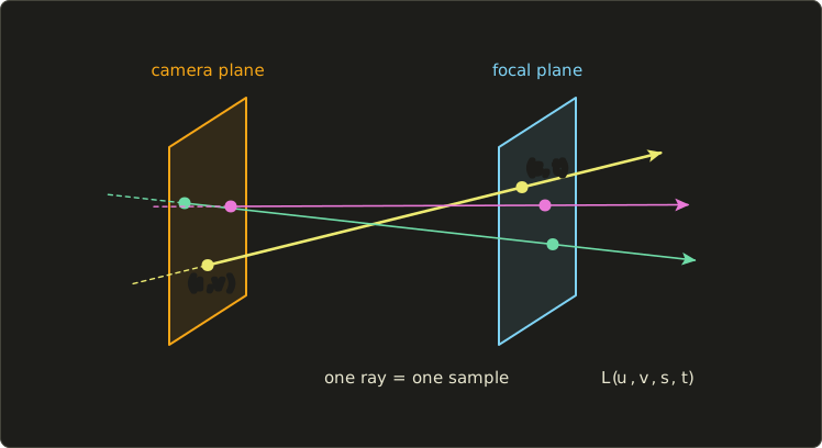
The light field is captured with a grid of cameras (or one camera moved over a grid) on the plane, each photo giving all for one .
A new view needs no geometry at all: for each pixel, compute its ray's and look the radiance up (interpolating between neighboring samples).
The Lumigraph adds an approximate geometry to improve that interpolation.
The cost is memory.
Worked example: camera positions with RGB pixels each is
for a single small object at a modest resolution, which is why both papers compressed the data heavily.
Light field cameras with a microlens array in front of the sensor capture a small light field in one shot and allow refocusing after the photo is taken.
Billboards and impostors
A cheaper relative of IBR is used in every game:
- A billboard (ビルボード) is a textured rectangle that always turns to face the camera: trees in the distance, particles of smoke and fire, grass.
- An impostor (インポスター) replaces a complex distant object by an image of it rendered on the fly or in advance; it is updated when the viewing angle has changed too much.
- Sprites in 2D games are the simplest image-based rendering of all.
From photos to models
IBR also works in the other direction: image-based modeling (イメージベーストモデリング) reconstructs geometry and textures from many photos, e.g. by photogrammetry (フォトグラメトリ); the input devices are covered in chapter 17.
The modern descendants of light fields learn a scene from photos and render new views: NeRF (neural radiance fields, 2020) stores the scene in a neural network that returns color and density for a position and direction, and 3D Gaussian splatting (2023) represents it as millions of small colored blobs that a rasterizer can draw in real time.
Part 2 covers them in its chapter on neural rendering.
Exam points
- IBR renders from images instead of (or besides) geometry; its classic techniques are IBL, panoramas, view interpolation and morphing, light fields and billboards.
- IBL needs HDR environment maps (light probes) because real light sources are far brighter than their surroundings.
- A panorama allows looking around from a fixed point but not moving.
- Plenoptic function: 7D (position 3, direction 2, wavelength, time); light field / lumigraph: 4D, because radiance is constant along rays in free space; two-plane parameterization .
12.14 Summary
- Local illumination uses only the light sources; global illumination also follows light via other surfaces: interreflection, color bleeding, reflection, refraction and caustics.
- Radiance (W/(m²·sr)) is light along a ray and stays constant along it in empty space; irradiance (W/m²) is light arriving at a surface. A uniform sky gives .
- The BRDF is outgoing radiance per incoming irradiance; it is reciprocal and energy conserving. A Lambertian surface has . Microfacet models (Cook–Torrance) multiply D, F and G.
- Fresnel: (0.04 for glass), Schlick ; every surface is a mirror at grazing angles.
- Snell: ; total internal reflection beyond the critical angle (41.81° for glass, 48.75° for water).
- Subsurface scattering (BSSRDF) makes skin and marble translucent; participating media absorb and scatter (Beer–Lambert ); Rayleigh scattering () makes the sky blue, Mie scattering makes clouds white; caustics are
LS+DEpaths. - The rendering equation: outgoing = emitted + integral of BRDF × incoming × cosine; it is recursive, and every method approximates it.
- Whitted ray tracing: primary, shadow, reflection and refraction rays in a ray tree; no diffuse interreflection, soft shadows, glossy reflection or caustics. Ray–sphere: .
- Acceleration: bounding volumes, BVH, uniform grids, octrees, kd-trees turn millions of tests into dozens.
- Distributed ray tracing spreads rays for soft shadows, glossy reflection, depth of field and motion blur; path tracing solves the rendering equation by Monte Carlo with noise , using importance sampling and Russian roulette.
- Radiosity: for diffuse patches; form factors depend only on geometry (); solved by Jacobi, Gauss–Seidel or progressive refinement; view independent, no specular.
- Photon mapping: photons from the lights stored in a photon map, then rendering with density estimation; good for caustics.
- Image-based rendering: IBL with HDR light probes, panoramas, view interpolation, morphing, 4D light fields (from the 7D plenoptic function), billboards and impostors; NeRF and Gaussian splatting are their modern descendants.
12.15 Key terms
| English | 日本語 |
|---|---|
| photorealistic rendering | 写実的表現(フォトリアリスティックレンダリング) |
| local illumination | 局所照明 |
| global illumination | 大域照明 |
| interreflection | 相互反射 |
| color bleeding | カラーブリーディング |
| caustics | コースティクス |
| light path notation | 光路の表記(ヘックバートの表記) |
| solid angle, steradian | 立体角、ステラジアン |
| radiant flux | 放射束 |
| radiant intensity | 放射強度 |
| irradiance | 放射照度 |
| radiance | 放射輝度 |
| BRDF | 双方向反射率分布関数 |
| reciprocity | 相反性 |
| energy conservation | エネルギー保存 |
| albedo | アルベド(反射率) |
| Lambertian surface | 完全拡散反射面(ランバート面) |
| glossy reflection | 光沢反射 |
| microfacet | マイクロファセット |
| Fresnel effect | フレネル効果 |
| Schlick's approximation | シュリックの近似 |
| refractive index | 屈折率 |
| Snell's law | スネルの法則 |
| total internal reflection | 全反射 |
| critical angle | 臨界角 |
| dispersion | 分散 |
| subsurface scattering | 表面下散乱 |
| translucent | 半透明 |
| participating media | 関与媒質 |
| Rayleigh scattering / Mie scattering | レイリー散乱/ミー散乱 |
| rendering equation | レンダリング方程式 |
| ray tracing | レイトレーシング法 |
| ray casting | レイキャスティング法 |
| primary ray / shadow ray | 一次レイ/シャドウレイ |
| reflection ray / refraction ray | 反射レイ/屈折レイ |
| ray tree | レイツリー |
| acceleration structure | 高速化データ構造 |
| bounding volume hierarchy (BVH) | 階層バウンディングボリューム(BVH) |
| uniform grid / octree / kd-tree | 均一格子/八分木/kd木 |
| distributed ray tracing | 分散レイトレーシング |
| Monte Carlo integration | モンテカルロ積分(モンテカルロ法) |
| path tracing | パストレーシング法 |
| importance sampling | 重点的サンプリング |
| Russian roulette | ロシアンルーレット |
| radiosity | ラジオシティ法 |
| patch | パッチ |
| form factor | 形態係数(フォームファクタ) |
| hemicube | ヘミキューブ |
| progressive refinement | 漸進的改良法 |
| view independent | 視点非依存 |
| photon mapping | フォトンマッピング法 |
| ambient occlusion | アンビエントオクルージョン(環境遮蔽) |
| image-based rendering (IBR) | イメージベーストレンダリング |
| image-based lighting (IBL) | イメージベーストライティング |
| high dynamic range (HDR) | 高ダイナミックレンジ(HDR) |
| light probe | ライトプローブ |
| panorama | パノラマ |
| view interpolation | 視点補間 |
| morphing | モーフィング |
| plenoptic function | プレノプティック関数 |
| light field | ライトフィールド(光線空間) |
| lumigraph | ルミグラフ |
| billboard / impostor | ビルボード/インポスター |
12.16 Challenges
- ★ Compute for diamond () and its critical angle against air. Then use Schlick to find the reflectance of water () at 80°, and the refraction angle of light going from water () into glass () at 30°.
- ★ A ray starts at in direction ; a sphere has center and radius 3. Find both values, the hit point, the unit normal and the reflected direction. (Check: the normal is a multiple of , and the reflected direction is a unit vector.)
- ★★ A path tracer shows 8% noise at 64 samples per pixel. How many samples does it need for 2%, and for 1%? A path with weight 0.3 meets Russian roulette with : list the possible weights afterwards with their probabilities and show that the expected weight is unchanged.
- ★★ Two patches face each other: patch 1 is a lamp with , , ; patch 2 has , , , and . Use reciprocity to find , solve the radiosity equations exactly, and do three Jacobi iterations starting from to watch them converge.
- ★★★ Classify these paths with Heckbert's notation and say which of Whitted ray tracing, radiosity, path tracing and photon mapping can render each: light through a window onto a matte floor, seen in a mirror; the reflection of a red wall in a chrome ball; a caustic from a glass seen through another glass. Then explain why a "radiosity first, ray tracing second" two-pass renderer still can't produce a caustic.
Multiple choice
Q1 ★ Which of the following statements about global illumination methods is correct?
| A | Whitted ray tracing computes color bleeding between matte surfaces because it follows shadow rays recursively. |
| B | Radiosity can render mirror reflections because the form factor contains the reflection direction. |
| C | Radiosity results depend on the camera position, so they must be recomputed every time the camera moves. |
| D | Radiosity computes the interreflection between diffuse surfaces and its result does not depend on the viewpoint. |
| E | Path tracing produces no noise as long as importance sampling is used. |
Q2 ★ Which of the following statements about the form factor in the radiosity method is correct?
| A | It depends on the albedo of patch . |
| B | For patch areas and , holds. |
| C | It increases in proportion to the distance between the two patches. |
| D | For a flat patch, . |
| E | It must be recomputed whenever the color of the light source changes. |
Q3 ★★ Which of the following statements about light field rendering is correct?
| A | It needs an exact 3D model of the object to synthesize a new view. |
| B | It is a 7-dimensional function of position, direction, wavelength and time. |
| C | It only allows rotating the view direction from a single fixed point, like a panorama. |
| D | It describes rays by their intersections with two concentric spheres. |
| E | Because radiance is constant along rays in free space, it describes the radiance of rays as a 4-dimensional function, e.g. by their intersections with two planes. |
12.17 Practical assignment
Trace one ray by hand through a small 2D scene, Whitted style, and then add the bounced light with radiosity.
You need graph paper (at least 26 × 16 squares, 1 square = 1 unit), a ruler, a protractor, a compass, a pencil, colored pens and a calculator.
The scene is a cross-section: the floor is the line , a glass disk (, so ) has center and radius 5, a point light is at with radiant intensity W/sr, and the eye is at , looking in the direction .
- Draw the floor, the disk, the light and the eye. Draw the primary ray.
- Intersect. Compute , , and the discriminant, and find the entry point . Compute the unit normal there and . Mark and draw the normal.
- Fresnel. Compute with Schlick. What fraction of the pixel comes from the reflection ray and what fraction from the refraction ray?
- Reflect. Compute and draw it. Does it hit the floor, or leave the scene? (If it leaves, it sees the black background.)
- Refract in. Compute with Snell's law and the refracted direction with the vector formula of section 12.5. Measure the angle on your drawing with the protractor. Find where leaves the disk (hint: the chord inside a circle has length ), compute the normal there, and refract out again (; check that there is no total internal reflection).
- Hit the floor. Find the point where the outgoing ray meets . Send a shadow ray from to the light and test it against the disk with the ray–circle formula. If it is unblocked, compute the irradiance at and the radiance of the floor with (Lambertian).
- Collect. Draw the ray tree of this pixel (eye, , reflection branch, refraction branches, shadow ray) and compute the pixel radiance as , ignoring the small loss at the second surface.
- Bounce. Now treat the lit floor around as patch 1 ( = the floor radiosity from step 6, ) and a wall patch facing it as patch 2 (, ), equal areas, . Do three Gauss–Seidel iterations and compare with the exact solution. By what percentage does the bounce raise the floor's radiosity?
How to check yourself: , and all have length 1; makes the angle with as Snell's law says; because a circle is symmetric, the ray leaves the disk at the same angle to the normal at which it entered (if your exit angle differs, look for a sign error); and add up to 1; and the radiosity iterations increase steadily towards the exact solution without overshooting it.
コメント(0)
まだコメントはありません。
ログインするとコメント出来ます。