23. Monte Carlo Rendering
In chapter 12 we met path tracing: shoot random paths from the eye, average them, and the rendering equation is solved, with noise that shrinks only as .
That chapter showed that it works and promised the details for Part 2.
This is that chapter.
We'll build Monte Carlo integration from the ground up (random variables, expectation, variance, the estimator), then the tools every production renderer uses to get clean images from fewer samples: inversion sampling, importance sampling (cosine, GGX, lights), stratified and quasi-Monte Carlo samples, and multiple importance sampling.
Then path tracing again, as an integral over paths, with throughput, Russian roulette, mirrors and a small C++ path tracer; the methods that go further (bidirectional, Metropolis, progressive photon mapping); bias and consistency; and finally denoising and adaptive sampling.
Part 2 goes beyond the exam syllabus, but this chapter deepens one of its items, global illumination (大域照明計算): path tracing, Monte Carlo integration, importance sampling and Russian roulette all appeared in chapter 12's exam points, and the first sections here explain exactly why they behave the way the exam expects.
You need the rendering equation, the BRDF and the light-path notation of chapter 12, and for section 23.5 the GGX distribution of chapter 22.
The math is school probability plus the integrals of chapter 12, which I'll always read out in words.
23.1 Why rendering needs random numbers
Remember the rendering equation of chapter 12 (section 12.7):
One pixel is not one evaluation of it.
A pixel's value is an integral over the pixel's area (anti-aliasing), over the lens (depth of field), over the shutter time (motion blur), and at every bounce over the hemisphere of incoming directions, and for soft shadows also over the area of the lamp.
Each of those adds dimensions: 2 for the pixel position, 2 for the lens, 1 for time, and per bounce 2 for the new direction and 2 for a point on the lamp.
Three bounces give
A grid with ten points per dimension needs evaluations, about three years for a GPU tracing a billion rays per second, for one pixel.
Worse, the trapezoid rule's error falls as in one dimension but only as in dimensions, because the points are spread over axes.
At that's : doubling the work improves the result by less than 9%.
This is the curse of dimensionality (次元の呪い).
Monte Carlo integration (モンテカルロ積分) breaks the curse.
Its error falls as whatever the dimension, it works with any number of samples, and it doesn't mind jumps in the integrand (shadow edges, silhouettes), where higher-order grid rules lose their advantage.
Above 4 dimensions it beats the trapezoid rule, and rendering lives far above 4.
The name comes from Los Alamos in the 1940s, where Stanisław Ulam, John von Neumann and Nicholas Metropolis used random sampling for neutron transport (Metropolis and Ulam, "The Monte Carlo Method", 1949), a close relative of light transport.
23.2 Probability in a nutshell
We need five ideas from probability, and only those.
Random variables and expectation
A random variable (確率変数) is a number that comes out of a random experiment: the result of a die roll, or the direction a path tracer picks.
Its expected value (期待値) is the average over infinitely many repetitions; for a fair die
Variance and standard deviation
The variance (分散) measures how far the values typically scatter around the mean: the expected squared distance from it.
For the die, , so .
The standard deviation (標準偏差) is its square root, , in the same units as itself.
In images, the standard deviation of a pixel's estimate is exactly what we see as noise (ノイズ).
(分散 is also the Japanese word for the dispersion of light in chapter 12.)
Continuous random variables
A direction or a position can be anything in a range.
Its probabilities are described by a probability density function (確率密度関数), the pdf : lands in a tiny interval around with probability .
A pdf is never negative, integrates to 1, and can be larger than 1 (a pdf squeezed into an interval of width 0.1 has height 10).
Its integral from the left end up to is the cumulative distribution function (累積分布関数), the CDF : the probability that .
Sums become integrals:
The simplest case is the uniform distribution on , , which is what a computer's random number generator gives us.
Its mean is and its variance is .
In this chapter (or for a concrete value) always means such a uniform random number.
Three rules
Three rules are all the error analysis needs:
- Expectation is linear: , always.
- Scaling scales the variance by the square: .
- For independent random variables, variances add: .
So averaging independent copies of a random variable with variance gives
The mean stays, the spread shrinks as : that is chapter 12's law, and it comes from the square in the second rule.
23.3 The Monte Carlo estimator
To estimate , draw independent samples with a pdf and compute
is an estimator (推定量): a random variable whose value is our guess for .
Dividing by is the important part: where samples are dense (large ) each one counts less, where they are sparse each one counts more.
Why it is right on average
One term has the expected value
The cancels, and by linearity the average of terms has the same expected value.
An estimator whose expected value is exactly the true value is unbiased (不偏).
The cancellation hides one condition: wherever ; a region that is never sampled is silently missing from the result.
How far off one estimate is
By the rules of section 23.2 the variance of is , where is the variance of one term:
Everything we do in the rest of this chapter to reduce noise is either making smaller (better , sections 23.5, 23.7, 23.8), making the samples not independent in a clever way (section 23.6), or removing noise after the fact (section 23.12).
Worked example: the area under a sine arch
The integral
has a known answer, so we can watch the estimator work.
Pick uniformly in , so and each term is .
With the four random numbers :
| u | x = πu | sin x | π sin x |
|---|---|---|---|
| 0.62 | 1.9478 | 0.9298 | 2.9210 |
| 0.35 | 1.0996 | 0.8910 | 2.7992 |
| 0.48 | 1.5080 | 0.9980 | 3.1354 |
| 0.81 | 2.5447 | 0.5621 | 1.7658 |
33% too high: three of the four samples landed near the top of the arch.
The expected scatter is
(using ).
With the standard deviation of is , so an error of 0.655 is unlucky but not unusual: about 1.4 standard deviations.
For large the estimates follow a bell curve (the central limit theorem), and about 95% of them fall within of the true value: for our sine with .
A renderer doesn't know , but it can estimate it from the samples themselves, which adaptive sampling (section 23.12) uses.
Exam points
This section ties to the global illumination item of the syllabus (chapter 12, section 12.10):
- The Monte Carlo estimator averages ; it is unbiased as long as wherever .
- Its standard deviation is : 4× the samples halve the noise, 100× the samples give one more correct digit.
- The rate doesn't depend on the dimension, which is why Monte Carlo is used for the high-dimensional integrals of global illumination.
23.4 Turning random numbers into samples
A computer gives us uniform numbers in .
Every other distribution has to be made from them.
The inversion method
The inversion method (逆関数法, inverse transform sampling) is the workhorse: compute the CDF , then set
Why does it work?
happens exactly when , and for a uniform that has probability .
So has the CDF , i.e. the pdf .
The recipe is always the same: integrate the pdf to get , set , solve for .
Example 1: distances in fog.
In a medium of density , the distance a photon flies before it interacts has the pdf (the Beer–Lambert law of chapter 12, section 12.6, read as a probability).
Then , and solving gives
With per meter and : m, the median free path.
Volumetric path tracers in chapter 28 use exactly this line.
Example 2: a tent.
We'll need the tent-shaped pdf on that rises linearly to a peak at and falls again:
(The triangle has base and height , so its area is 1.)
On the left half , which reaches at the peak; solving gives for , and by symmetry for .
When can't be inverted, rejection sampling (棄却法) is the fallback: draw candidates in a simple region around the shape and discard those outside.
For a point in the unit disk, draw in the square and keep it if ; the disk covers of the square, so a point costs 1.27 candidates on average, and the varying loop count is why GPUs prefer inversion.
Directions on the hemisphere
A direction on the hemisphere around the normal is described by the polar angle (from the normal) and the azimuth (around it).
A small patch of directions has the solid angle : rings near the horizon are longer than rings near the pole.
For a pdf over solid angle, the pdf over is therefore , and we can sample and separately by inversion.
Uniform hemisphere (半球上の一様サンプリング): .
The pdf of is , its CDF is , so (or just , since is uniform too), and .
So is uniform in , as chapter 12 used.
Cosine-weighted hemisphere (コサイン重み付き半球サンプリング): (the normalizes it, because ).
The pdf of is , its CDF is , so
In local coordinates (normal = z axis) that's : a uniform point in the unit disk lifted straight up onto the hemisphere (Malley's method).
Worked example: , give , (), , the direction and the pdf per steradian.
In the scene the local direction becomes in a frame built around the normal with two cross products (Linear Algebra chapter 5), as the C++ path tracer of section 23.9 does.
In a shader, with two helpers for sections 23.7 and 23.8:
static const float PI = 3.14159265;

// Cosine-weighted direction in the local frame (z = normal); pdf = cos(theta) / pi.
float3 sampleCosine(float2 u) {
  float r = sqrt(u.x);
  float phi = 2.0 * PI * u.y;
  return float3(r * cos(phi), r * sin(phi), sqrt(max(0.0, 1.0 - u.x)));
}

// Solid-angle pdf of a point picked uniformly on a light of area A (section 23.7).
float lightPdf(float dist, float cosLight, float area) {
  return dist * dist / (area * cosLight);
}

// Power heuristic (beta = 2): MIS weight of technique a against technique b (section 23.8).
float powerHeuristic(float pdfA, float pdfB) {
  float a = pdfA * pdfA;
  float b = pdfB * pdfB;
  return (a + b) > 0.0 ? a / (a + b) : 0.0;
}
const float PI = 3.14159265;
// Cosine-weighted direction in the local frame (z = normal); pdf = cos(theta) / pi.
vec3 sampleCosine(vec2 u) {
float r = sqrt(u.x);
float phi = 2.0 * PI * u.y;
return vec3(r * cos(phi), r * sin(phi), sqrt(max(0.0, 1.0 - u.x)));
}
// Solid-angle pdf of a point picked uniformly on a light of area A (section 23.7).
float lightPdf(float dist, float cosLight, float area) {
return dist * dist / (area * cosLight);
}
// Power heuristic (beta = 2): MIS weight of technique a against technique b (section 23.8).
float powerHeuristic(float pdfA, float pdfB) {
float a = pdfA * pdfA;
float b = pdfB * pdfB;
return (a + b) > 0.0 ? a / (a + b) : 0.0;
}static const float PI = 3.14159265;
// Cosine-weighted direction in the local frame (z = normal); pdf = cos(theta) / pi.
float3 sampleCosine(float2 u) {
float r = sqrt(u.x);
float phi = 2.0 * PI * u.y;
return float3(r * cos(phi), r * sin(phi), sqrt(max(0.0, 1.0 - u.x)));
}
// Solid-angle pdf of a point picked uniformly on a light of area A (section 23.7).
float lightPdf(float dist, float cosLight, float area) {
return dist * dist / (area * cosLight);
}
// Power heuristic (beta = 2): MIS weight of technique a against technique b (section 23.8).
float powerHeuristic(float pdfA, float pdfB) {
float a = pdfA * pdfA;
float b = pdfB * pdfB;
return (a + b) > 0.0 ? a / (a + b) : 0.0;
}23.5 Importance sampling
Look at the variance formula of section 23.3 again: .
If we could choose (for a positive ), every term would be exactly, and the variance would be zero.
We can't, because that needs , the answer we're looking for.
But it tells us the direction: the more the pdf looks like the integrand, the less noise.
Choosing that way is importance sampling (重点的サンプリング); chapter 12 showed its most extreme case, cosine sampling of .
Worked example: the sine again
For , three choices of :
| shape | each term | variance per sample σ² | |
|---|---|---|---|
| uniform, | flat | 0.9348 | |
| tent (section 23.4) | roughly like sin | 0.0670 | |
| exactly like sin | always 2 | 0 |
The tent's variance, (numerically), is 14 times smaller: 14 times fewer samples for the same noise.
The same four random numbers through the tent's inverse CDF:
| u | x | sin x | p(x) | sin x / p(x) |
|---|---|---|---|---|
| 0.62 | 1.7722 | 0.9798 | 0.5550 | 1.7654 |
| 0.35 | 1.3142 | 0.9673 | 0.5326 | 1.8160 |
| 0.48 | 1.5391 | 0.9995 | 0.6238 | 1.6024 |
| 0.81 | 2.1733 | 0.8239 | 0.3924 | 2.0995 |
9% low instead of 33% high, and all four terms are close to 2.
The ideal pdf is sampled by inversion as , and every sample gives exactly 2.
The danger: a pdf that is too small
Importance sampling can also make things much worse.
Take a V-shaped pdf , the tent upside down: it is zero exactly at the peak of the sine.
It is positive almost everywhere, so the estimator is still unbiased, but near the terms explode and diverges: the variance is infinite.
samples still average to 2.000, but the sample variance (32 in my run) never settles; in an image that means rare, extremely bright pixels.
The rule: may be too large where is small (that only wastes samples), but it must never be much too small where is large.
Importance sampling in a renderer
The integrand of the rendering equation is a product .
The incoming light is unknown (it's what the recursion computes), so we importance sample the factors we know:
- BSDF sampling (BSDFサンプリング): as closely as possible. For a Lambertian surface that's cosine sampling, and .
- Light sampling (光源サンプリング): the light that arrives directly from the lamps (section 23.7).
- Environment map sampling: invert a 2D table of the HDR sky's brightness (chapter 12, section 12.13), a CDF over rows and then over the pixels of the chosen row, so that the sun gets most of the samples.
For chapter 12's irradiance from a uniform sky, uniform hemisphere sampling gives terms with , cosine sampling gives every time.
Sampling the GGX lobe
A glossy microfacet BRDF (chapter 22) is concentrated around the mirror direction, where cosine sampling sends almost no samples.
The classic approach (Walter, Marschner, Li and Torrance, 2007) samples the half vector (the microfacet normal) from the GGX distribution and reflects the view direction about it.
With the GGX width parameter (many engines set ):
This pdf integrates to 1 over the hemisphere (that's how is normalized), and inverting its CDF gives
Then , and because reflecting about doubles angles, the pdf in terms of picks up a Jacobian:
Worked example. , looking straight down the normal (), :
( here, so .)
The reflected direction leaves at from the normal.
Half of all half vectors fall within 16.70° of the normal, and 90% within 41.99° (): the lobe is sampled, the empty hemisphere isn't.
Today's refinement samples only the normals the viewer can actually see (VNDF sampling, Eric Heitz, 2018), which matters most at grazing angles.
What it looks like
Here is the box of chapter 12, path traced with the same number of samples (16 per pixel) and three sampling strategies at each diffuse bounce, with the RMS error against a reference of 2048 samples per pixel:
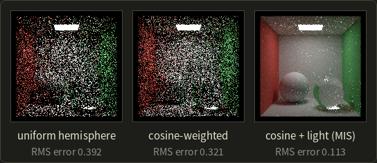
Cosine sampling lowers the error by 18%: it matches one factor of the integrand.
The big jump comes from also sampling the lamp directly (section 23.7), because most of the noise in the first two images comes from paths that find the small lamp only by luck.
23.6 Stratified sampling and quasi-Monte Carlo
Importance sampling changes where samples go on average; the other lever is how evenly they are spread.
Independent random samples clump and leave gaps, like three of the four samples of section 23.3 near the top of the arch.
Stratified sampling
Stratified sampling (層化サンプリング) divides the domain into equal pieces (strata) and puts one random sample into each.
In one dimension, sample (counting from 0) is .
With our four numbers:
| k | (k + u)/4 | x | π sin x |
|---|---|---|---|
| 0 | 0.1550 | 0.4869 | 1.4700 |
| 1 | 0.3375 | 1.0603 | 2.7410 |
| 2 | 0.6200 | 1.9478 | 2.9210 |
| 3 | 0.9525 | 2.9924 | 0.4671 |
, 5% low.
Every quarter of the arch got exactly one sample, so no clumping is possible.
The estimate stays unbiased, and its variance is never larger than with independent samples.
For a smooth function the error falls as in one dimension and as in dimensions.
The regular supersampling grid of chapter 2 (section 2.7) becomes stratified sampling when each sample is moved randomly inside its cell, which is called jittered sampling (ジッターサンプリング).
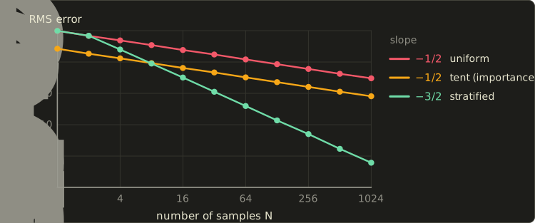
The measured RMS errors (4000 runs per point) follow the predictions: at 1024 samples, 0.030 for uniform (), 0.0081 for the tent () and 0.00006 for stratified sampling.
Importance sampling shifts the line down, stratification makes it steeper, and the two combine: stratify the values, then push them through the inverse CDF.
The catch is dimensionality again.
A full jittered grid in dimensions needs samples: 2 strata per axis in 17 dimensions is 131,072 samples per pixel.
Renderers therefore stratify small groups of dimensions separately (pixel, lens, each bounce) and shuffle the pairing between groups, the idea behind Latin hypercube and multi-jittered sampling.
Quasi-Monte Carlo
Quasi-Monte Carlo (準モンテカルロ法, QMC) drops randomness altogether and uses deterministic low-discrepancy sequences (低食い違い量列) designed to fill space evenly for any number of points.
The discrepancy (食い違い量) of a point set is its worst unevenness: over all boxes anchored at the origin, the largest difference between the fraction of points inside and the box's volume.
The Koksma–Hlawka inequality bounds the error by (variation of ) × (discrepancy), and good sequences reach about , almost .
The building block is the radical inverse (ラディカルインバース) in base : write the index in base and mirror its digits around the point.
In base 2: , , , .
The base-2 sequence is the van der Corput sequence (ファン・デル・コルプット列): each new point lands in one of the largest remaining gaps.
The Halton sequence (ハルトン列; John Halton, 1960) uses a different prime base per dimension: point is (radical inverse of in base 2, in base 3, in base 5, …).
Worked example, point 6 in 2D: base 2 gives 0.375 as above, and , so the point is .
The first eight base-3 values are .
The Sobol sequence (ソボル列; Ilya Sobol, 1967) works in base 2 in every dimension, with different "direction numbers" per dimension combined by XOR.
It stays good in far more dimensions than Halton (whose large bases form regular stripes) and is fast with bit operations, so production renderers usually prefer it.
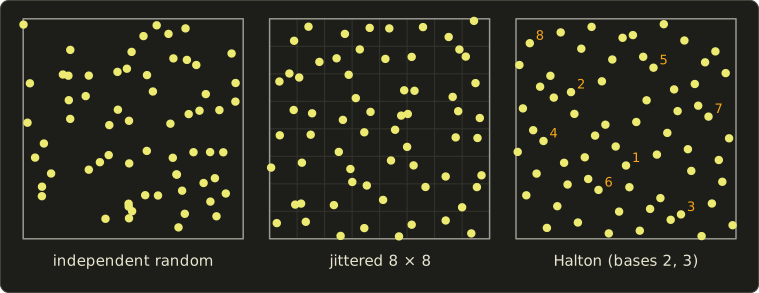
A deterministic sequence gives no error estimate.
Randomized QMC adds the same random offset to every point and wraps around (the Cranley–Patterson rotation), or randomly permutes the digits (Owen scrambling): each point is then uniform, so the estimator is unbiased again, and the points keep their even spread.
For the smooth 2D integrand , the measured RMS errors over 2000 randomizations are:
| N | independent random | jittered grid | Halton, randomly shifted |
|---|---|---|---|
| 16 | 0.0414 | 0.0109 | 0.0180 |
| 64 | 0.0209 | 0.00269 | 0.00473 |
| 256 | 0.0102 | 0.00069 | 0.00132 |
| 1024 | 0.0052 | 0.00017 | 0.00041 |
At 1024 samples the shifted Halton points are 13 times more accurate than random ones.
The jittered grid wins here only because is a perfect square in 2D; Halton points work for every , can be extended one sample at a time, and scale to many dimensions.
Real-time renderers with one or two samples per pixel care more about how the remaining error looks: blue noise (ブルーノイズ) patterns turn it into fine grain that the eye and a denoiser handle better than clumps.
23.7 Sampling the lights
Why did cosine sampling still produce so much noise? Because the lamp is small, and a cosine-sampled direction rarely hits it.
How often does a random bounce find the lamp?
Take a point on the floor 2 m right below the center of a square lamp of 0.6 m × 0.6 m ( m², the lamp of chapter 12's box) with radiance .
The irradiance from the lamp, integrated numerically, is W/m².
A cosine-sampled direction hits the lamp with probability
Only 2.8% of the bounces see the lamp, so an estimate is either 0 or large, the worst kind of noise.
For a point light (zero solid angle) the probability is exactly 0.
Sampling a point on the light
Light sampling turns this around: pick a point on the lamp uniformly over its area () and send a shadow ray to it.
This is next event estimation (次イベント推定, NEE), which chapter 12's path tracer already did.
Directions and lamp area are related by the geometry in this picture:
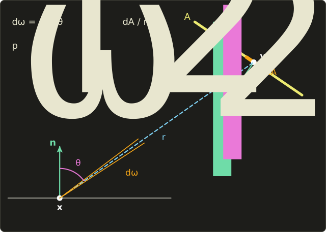
A patch looks smaller from far away and when tilted, as in chapter 12's solid angle.
So a pdf of over the area is, in solid angle at ,
and the direct-light estimator with one sample is
with = 1 if the shadow ray is free, 0 if blocked.
Worked example. The floor point under the lamp, white floor with , so .
A sample at the lamp's center: , both cosines are 1, and the irradiance part is .
A sample at a corner relative to the floor point: , , and the irradiance part is .
Every sample lands between these two values, close to the true 1.2234, against "0 or 36 times too much" for cosine sampling.
The reflected radiance from the center sample is (true value ).
In solid-angle terms the light pdf toward the center is per steradian, while cosine sampling has there: 35 times more samples go to where the light is.
Many lights
With thousands of lamps, pick one at random with probability and divide its contribution by , the rule one level up.
Proportional to power, lamps of 100, 50 and 10 W get ; the weak lamp's contribution, when picked, is multiplied by 16.
Production renderers pick lights from a tree (a "light BVH") that favors bright and close lights, and ReSTIR (chapter 24) reuses good light samples across pixels and frames to handle millions of lights in real time.
23.8 Multiple importance sampling
Light sampling is great for a matte floor under a small lamp.
Now make the floor nearly a mirror and the lamp a huge window: light samples spread over the window, almost all outside the sharp BRDF lobe (value nearly 0) and a rare one inside (huge value), while BSDF sampling sends every ray into the lobe, where it hits the window easily.
Which technique wins depends on material and light, and a real scene has every combination at once.
Combining two techniques
Multiple importance sampling (多重重点的サンプリング, MIS), introduced by Eric Veach and Leonidas Guibas in 1995 ("Optimally Combining Sampling Techniques for Monte Carlo Rendering"), uses both techniques and weights each sample by how good its technique is at that point.
With samples from technique with pdf :
This is unbiased as long as, at every where , the weights add up to 1, (and where ).
The proof is one line: the expected value is .
The question is how to choose the weights.
Veach and Guibas proposed two heuristics:
usually with .
A technique with a high pdf at the point (it finds such points often) gets a large weight; a sample found only by luck (low pdf, huge ) gets a small one, and that is exactly the sample that would otherwise be a firefly.
With the balance heuristic each term becomes , as if all samples came from one mixed pdf, and Veach proved its variance exceeds that of any other weighting by at most .
The power heuristic sharpens the weights, which helps when one technique is clearly right, and is what most renderers use.
Worked example: weights
The matte floor of section 23.7, a direction toward the lamp's center, one sample from each technique: , .
Light sampling is clearly right here, and MIS gives it nearly all the weight.
A glossy surface with the same kind of lamp, where at some direction and :
In both cases each pair of weights adds up to 1, which is what keeps the estimator unbiased.
Worked example: variance
A one-dimensional "flatland" version makes the effect measurable.
A glossy lobe (a bell curve of width around 20°, followed exactly by BSDF sampling) is lit by a lamp covering an interval of angles (sampled uniformly by light sampling); the integrand is lobe × cosine inside the lamp.
Exact relative standard deviations (standard deviation / true value) for two cases, with 2 samples in total (2 of one technique, or 1 + 1 with MIS):
| case | BSDF sampling only | light sampling only | MIS balance | MIS power |
|---|---|---|---|---|
| broad lobe (s = 30°), small lamp (10°) | 180% | 1.3% | 30% | 4.8% |
| sharp lobe (s = 3°), large lamp (60°) | 1.4% | 152% | 34% | 22% |
Each single technique is excellent in one case and terrible in the other.
MIS is never terrible: it loses something against the right technique (which got 2 samples instead of 1) but removes the 150–180% catastrophes, and the power heuristic beats the balance heuristic in both cases.
A renderer doesn't know which case each pixel is, so that robustness is what it needs.
Here are the two pdfs and the weights for an in-between case (lobe width 12° around 0°, lamp from −5° to 35°):
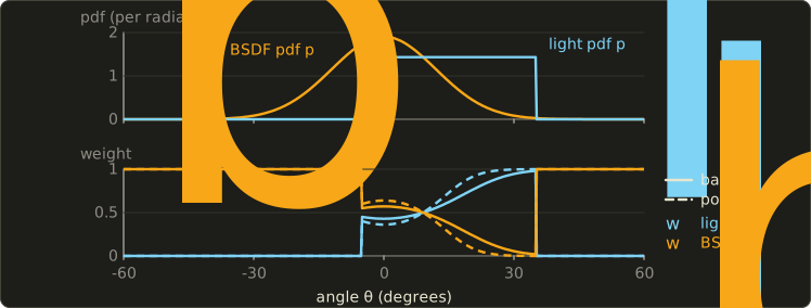
Where the lobe is high BSDF sampling gets the weight, towards its edge light sampling takes over, and the weights cross at 9°, exactly where .
MIS also has a one-sample form: pick technique with probability , draw one sample and use , handy for choosing between the layers of a material (diffuse base or clear coat).
23.9 Path tracing in depth
To reason about what a path tracer estimates, and to build the methods of section 23.10, Veach's thesis ("Robust Monte Carlo Methods for Light Transport Simulation", Stanford, 1997) rewrote the rendering equation as an ordinary integral over paths.
The path integral
A path of length is a list of points : on the camera, on a light, the others on surfaces.
The value of pixel is
an integral over all vertex positions, for every path length.
The measurement contribution function multiplies the emitted light, the BSDF at every bounce, the camera's sensitivity , and between consecutive vertices a geometry term (幾何項):
is the area-to-area version of section 23.7's : how well two points "see" each other.
Two points 2 m apart with cosines 0.8 and 0.6 and no occlusion have per m² (the radiosity form factor of chapter 12 is this divided by and averaged over two patches).
Heckbert's notation now has a precise meaning (LDSE is the set of paths with vertices light, diffuse, specular, eye), and every rendering algorithm is a way to sample paths and divide by the density of having produced them.
Throughput
A path tracer chooses a direction at each vertex, not a point.
A direction with solid-angle pdf gives the next vertex the area pdf (section 23.7 again), which cancels against the same factors in , leaving the throughput (スループット) update:
starts at 1 at the camera; whenever the path reaches emitted light , the pixel gets .
For a Lambertian surface with cosine sampling the factor is the albedo (section 23.5), so after diffuse bounces .
Russian roulette, with its cost
Stopping paths at a fixed maximum depth is biased: light that needs more bounces is lost.
Russian roulette (ロシアンルーレット, brought to graphics by James Arvo and David Kirk in 1990) continues with probability and divides by , otherwise stops; a remaining contribution becomes with probability and 0 otherwise:
Unbiased, but not free: the added variance is
With chapter 12's example (, ) that's , in exchange for skipping 30% of the work.
What counts is efficiency (効率), : roulette pays off when it kills paths with small remaining contributions.
Hence the usual after a few bounces: dim paths are culled, survivors are lifted back to a throughput near 1, and with a constant a path makes bounces on average (5 for ).
A tiny path tracer
Here is the core loop of a path tracer in C++, in a scene whose answer we know: the camera sits inside a closed sphere whose inner wall is Lambertian with albedo and emits radiance .
By chapter 12's geometric series (section 12.7) the exact answer is , 5 for .
The loop intersects the sphere, adds the emission times the throughput, samples a cosine-weighted direction, multiplies the throughput by and plays Russian roulette, using Vec3, dot, cross and normalize from the Linear Algebra series' linalg.hh:
#include <algorithm>
#include <cmath>
#include <cstdio>
#include <random>
#include "linalg.hh"

// A camera at the center of a closed sphere (radius 1). The inside wall is
// Lambertian with albedo rho and emits radiance Le. Exact answer: Le / (1 - rho).
const float PI = 3.14159265f;
std::mt19937 gen(7);
float rnd() { return (gen() >> 8) * (1.0f / 16777216.0f); }

// Cosine-weighted direction around the unit normal n (pdf = cos / pi).
Vec3 sampleCosine(Vec3 n) {
  float u1 = rnd(), u2 = rnd();
  float r = std::sqrt(u1), phi = 2.0f * PI * u2;
  Vec3 a = std::fabs(n.x) > 0.9f ? Vec3{0, 1, 0} : Vec3{1, 0, 0};
  Vec3 t = normalize(cross(a, n));
  Vec3 b = cross(n, t);
  return r * std::cos(phi) * t + r * std::sin(phi) * b + std::sqrt(1.0f - u1) * n;
}

// The core loop of a path tracer. maxDepth < 0 means: no limit, Russian roulette instead.
float radiance(Vec3 o, Vec3 d, float rho, float Le, int maxDepth, int *bounces) {
  float L = 0.0f, beta = 1.0f;  // beta = path throughput
  for (int depth = 0;; depth++) {
    float b = dot(o, d), c = dot(o, o) - 1.0f;  // hit the sphere from inside
    Vec3 p = o + (-b + std::sqrt(b * b - c)) * d;
    Vec3 n = -1.0f * p;                         // inward unit normal
    L += beta * Le;                             // emission at the hit
    *bounces = depth + 1;
    if (maxDepth >= 0 && depth >= maxDepth) break;
    d = sampleCosine(n);
    beta *= rho;                                // f cos / p = (rho/pi) cos / (cos/pi)
    if (maxDepth < 0) {                         // Russian roulette
      float q = std::min(beta, 1.0f);
      if (rnd() >= q) break;
      beta /= q;
    }
    o = p + 1e-4f * n;
  }
  return L;
}

void run(const char *name, float rho, int maxDepth) {
  const int paths = 1000000;
  double sum = 0, sq = 0, steps = 0;
  for (int i = 0; i < paths; i++) {
    int k = 0;
    double v = radiance({0, 0, 0}, {0, 0, -1}, rho, 1.0f, maxDepth, &k);
    sum += v;
    sq += v * v;
    steps += k;
  }
  double mean = sum / paths, sd = std::sqrt(std::max(0.0, sq / paths - mean * mean));
  printf("%-22s mean = %.4f  sd per path = %.3f  hits per path = %.3f\n", name, mean, sd, steps / paths);
}

int main() {
  float rho = 0.8f;
  printf("exact Le / (1 - rho)   = %.4f\n", 1.0f / (1.0f - rho));
  run("max depth 4", rho, 4);
  run("max depth 16", rho, 16);
  run("Russian roulette", rho, -1);
  return 0;
}
exact Le / (1 - rho)   = 5.0000
max depth 4            mean = 3.3616  sd per path = 0.000  hits per path = 5.000
max depth 16           mean = 4.8874  sd per path = 0.000  hits per path = 17.000
Russian roulette       mean = 5.0006  sd per path = 4.478  hits per path = 5.001
Bias and variance in three lines.
Stopping after 5 hits is noise-free in this symmetric scene but 33% too dark (); after 17 hits it is still 2% too dark ().
Russian roulette is right on average (5.0006, with a standard error of for a million paths) at 5 hits per path, , but each path is noisy: its value is its number of hits, a geometric random variable with standard deviation .
This is chapter 12's white furnace test (section 12.13), which every serious renderer runs.
Mirrors and glass: delta distributions
A perfect mirror's BRDF is a delta distribution (デルタ分布): zero everywhere except in one direction, with total (the Fresnel reflectance).
The path tracer takes the mirror direction and replaces by its limit (or by 1 when it chooses reflection or refraction with probabilities and , as chapter 12's renderer does).
Light sampling can't help there (a random lamp point is exactly in the mirror direction with probability 0), so specular vertices skip NEE, and a lamp hit right after a specular bounce counts with MIS weight 1; in this chapter's renderer that's one flag.
This explains chapter 12's stubborn speckles under the glass ball: a caustic path LSDE traced from the eye must bounce off the floor, pass the glass and hit the small lamp by chance, and with a point light it can't happen at all.
Paths LS+DS+E (a caustic seen in a mirror, a pool floor seen through the water) are the hardest for any method that connects at a diffuse vertex.
MIS inside the path tracer
Combining sections 23.7 and 23.8, every non-specular vertex does two things:
at a diffuse or glossy vertex x (throughput beta, outgoing direction wo):
    light sample:  pick y on a light, pdf pL (solid angle)
                   if visible: add beta * f(wo, wi) * cos * Le / pL * w(pL, pB(wi))
    BSDF sample:   pick wi with pdf pB, beta *= f(wo, wi) * cos / pB
                   trace the ray; if it hits a light:
                       add beta * Le * w(pB, pL(hit))
                   otherwise continue the path from the hit
w(a, b) is the power heuristic of section 23.4's snippet; this is the "cosine + light (MIS)" renderer of the figure in section 23.5.
23.10 Bidirectional methods, Metropolis and photon mapping
Path tracing with MIS is the standard in film production, but caustics from small lights, light entering through a gap and light seen through glass stay hard; here are the ideas of the main alternatives.
Bidirectional path tracing
Bidirectional path tracing (双方向パストレーシング, BDPT; Eric Lafortune and Yves Willems, 1993, and independently Veach and Guibas, 1994) traces one subpath from the camera and one from a light, then connects vertices of the two with a shadow ray:
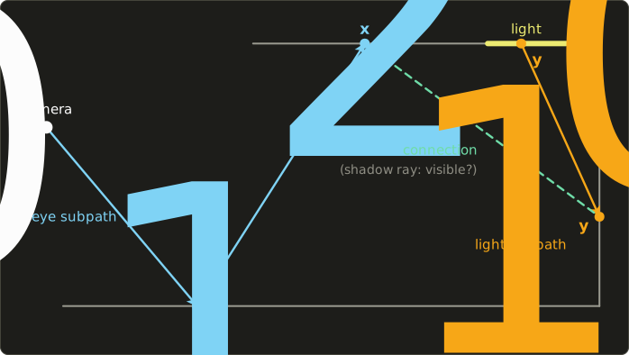
The same complete path can be produced in several ways: with vertices from the light side and from the eye side, a path with vertices can be built in ways ( with ).
For the 5 vertices in the picture () that's 6 techniques: is pure path tracing (the eye path hits the lamp by itself), is path tracing with next event estimation, is the connection drawn, and so on up to , a light path that hits the camera by itself (impossible for a pinhole camera, so its pdf is 0).
MIS over all pdfs combines them; this is the setting MIS was invented for.
The technique , connecting light vertices directly to the camera, is light tracing (ライトトレーシング), which renders directly seen caustics (LS+DE) easily.
The price is complexity and more work per sample.
Metropolis light transport
Some paths are rare even for BDPT, like light through a door left ajar.
Metropolis light transport (メトロポリス光輸送, MLT; Veach and Guibas, 1997) applies the Metropolis–Hastings algorithm (1953, 1970): once a path that carries light is found, explore its neighborhood.
It builds a Markov chain (マルコフ連鎖) of paths: from the current path propose a mutation (変異) (move a vertex, replace a subpath…) and accept it with probability
where is the path's brightness and the probability of proposing one path from the other.
For a symmetric mutation the s cancel: going from a path of brightness 2 to one of 0.5 is accepted with probability , to one of 3 always.
The chain visits paths in proportion to their brightness, and a separate ordinary estimate of the total image brightness sets the scale.
Consecutive samples are correlated, so noise is blotchy and convergence uneven, and the start of the chain biases the result early on.
Primary sample space MLT (Csaba Kelemen and colleagues, 2002) simplified it greatly by mutating the random numbers that drive an ordinary path tracer.
Photon mapping, progressive
Chapter 12's photon mapping estimates radiance from the photon density , which blurs over the radius : it is biased, and only consistent if the photon count goes to infinity while goes to zero, impossible with one stored photon map.
Progressive photon mapping (プログレッシブフォトンマッピング; Toshiya Hachisuka, Shinji Ogaki and Henrik Wann Jensen, 2008) runs any number of photon passes without storing them.
Each eye-ray hit point keeps a radius and a count ; after a pass finds new photons inside, it keeps a fraction of them and shrinks the disk so the density stays the same:
The paper uses .
Worked example: , : and .
The radius shrinks with every pass, the bias goes to zero, and the image converges, including the SDS paths that defeat path tracing.
Stochastic progressive photon mapping (Hachisuka and Jensen, 2009) extends it to glossy reflections and depth of field, and in 2012 two groups combined photon density estimation with BDPT under MIS: vertex connection and merging (VCM; Iliyan Georgiev and colleagues) and unified path sampling (UPS; Hachisuka and colleagues).
Volumes add scattering vertices inside the medium, with the free-flight sampling of section 23.4 (chapter 28).
| method | bias | strong at | weak at |
|---|---|---|---|
| path tracing + NEE + MIS | unbiased | most scenes, simple | caustics, small openings |
| bidirectional path tracing | unbiased | direct caustics, indirectly lit rooms | SDS paths, cost per sample |
| Metropolis light transport | unbiased in the limit | very hard visibility | blotchy, uneven convergence |
| photon mapping (fixed map) | biased, not consistent | caustics, SDS |
blur, memory |
| progressive photon mapping | biased, consistent | caustics, SDS, bounded memory |
slow on diffuse light |
23.11 Bias, variance and consistency
Three words need pinning down.
- Bias (バイアス、偏り): , the error that remains on average. An estimator with zero bias is unbiased.
- Variance: the random scatter around , visible as noise.
- Consistent (一致性がある): the error goes to zero as the work (samples, photons, passes) goes to infinity. An unbiased estimator with finite variance is consistent; a biased one can be consistent if its bias shrinks with the work.
What we really see is the total error, measured by the mean squared error (平均二乗誤差, MSE):
Worked example. At the same render time, renderer A is unbiased with variance 0.04, renderer B has a bias of 0.05 and variance 0.01.
A: MSE = 0.04. B: MSE = , about three times better.
Render 16 times longer: A's MSE drops to , B's to because its bias stays (if B isn't consistent), and A wins from then on.
Biased methods (photon mapping, clamping, denoising) look good quickly; unbiased ones win in the limit and are easier to trust, because their error can be estimated from the samples.
| technique | biased? | consistent? |
|---|---|---|
| path tracing, BDPT (with Russian roulette) | no | yes |
| a fixed maximum path depth | yes (too dark) | no |
| Russian roulette | no (adds variance) | yes |
| photon mapping, fixed photon map | yes (blur) | no |
| progressive photon mapping | yes | yes |
| clamping sample values | yes (too dark) | no |
| denoising with a fixed filter | yes (blur) | no |
Fireflies and clamping
A firefly (ファイアフライ) is a single pixel far brighter than its neighbors: one sample with a tiny pdf and a large , typically a caustic found from the eye.
Take a pixel whose samples are 0.5 with probability 99.9% and 500 with probability 0.1%:
Half of the true brightness comes from the rare path.
One sample has , a variance of , a standard deviation of 15.8, and at 64 samples per pixel still , twice the pixel's value.
What we see: of such pixels catch a rare sample and show about , a white dot; the other 93.8% show 0.5, half as bright as they should be.
Clamping (クランプ) limits every sample to a maximum, say 10.
The fireflies are gone, but the mean is now instead of 0.9995, whatever the number of samples.
Production renderers clamp anyway (often only indirect light, as the denoising figure below does), because missing caustic brightness bothers viewers less than speckles; the real fix is a technique that finds those paths often (section 23.10).
23.12 Denoising and adaptive sampling
Film frames still need hundreds to thousands of samples per pixel, and a game frame can afford about one.
Denoising (デノイズ) closes the gap by filtering the noisy image, and to avoid blurring edges and textures it uses information the renderer has for free.
Using the G-buffer
The renderer knows each pixel's normal, position or depth, and albedo at the first hit, the G-buffer (Gバッファ) of a deferred renderer; these are nearly noise-free and show exactly where the edges are.
A cross-bilateral filter (クロスバイラテラルフィルタ), the bilateral filter of chapter 15 with edge weights taken from other images, averages a pixel only with neighbors of similar normal, position and color.
Two more tricks:
- Demodulate the albedo (アルベドの分離): divide the color by the albedo before filtering and multiply it back after, so the filter smooths the lighting and leaves the texture sharp.
- Keep the emitters out: a directly seen lamp isn't noisy and must not be smeared into its surroundings.
The edge-avoiding à-trous filter
Low sample counts need a wide filter, and a 65 × 65 cross-bilateral window costs 4,225 taps per pixel.
The edge-avoiding à-trous wavelet transform (Holger Dammertz, Daniel Sewtz, Johannes Hanika and Hendrik Lensch, 2010) applies a 5 × 5 filter several times with the taps spread twice as far each time ("à trous" is French for "with holes"):
- the 1D weights are the B3-spline , and the 5 × 5 kernel is their product, 25 taps;
- pass (from 0) uses taps pixels apart, so the fifth pass reaches pixels to each side, a 65 × 65 window;
- every tap's weight is multiplied by edge-stopping weights (エッジ停止関数) from the color, normal and position differences, so the filter never reaches across an edge.
Five passes cost taps per pixel instead of 4,225, and the paper halves the color tolerance after each pass, as the noise left gets smaller.
Worked example: one tap's weight.
A neighbor in the second pass at kernel offset (+1, 0), 2 pixels to the right, has the spline weight .
SVGF's edge-stopping functions (below) multiply it by a normal weight and a luminance weight , with the local standard deviation of the noise.
For the normal weight is ; across a crease with it is , effectively zero.
A luminance difference of 0.1 with gives , and the tap's weight is before normalization.
SVGF: adding time and variance
Spatiotemporal variance-guided filtering (SVGF; Christoph Schied and colleagues at NVIDIA and KIT, 2017) turned this into a real-time denoiser for one sample per pixel:
- Temporal accumulation (時間方向の蓄積): reproject last frame's result with motion vectors and blend, with . This moving average reduces the noise variance to , like averaging 9 frames; disocclusions reset the history.
- Variance estimation: per-pixel luminance variance from moments accumulated over time (spatially where the history is short).
- À-trous filtering: 5 passes with normal, depth and variance-guided luminance weights, so noisy regions are smoothed hard and converged ones barely touched; the variance is filtered along with the color.
With albedo demodulated, the paper reports about 10 ms at 1920 × 1080 on the GPUs of the time.
Here is the box scene at 8 samples per pixel (indirect light clamped at 2), filtered by a Gaussian blur and by an à-trous filter in this spirit (5 passes; normal, position and material edge stopping; luminance weights guided by a spatial variance estimate; albedo demodulated; lamp kept out), with RMS errors measured on the displayed sRGB values:
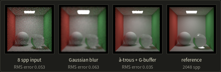
The Gaussian blur is worse than the input: it trades noise for blur everywhere and makes the lamp glow.
The edge-aware filter cuts the error by a third and keeps the geometry sharp, but the caustic under the glass ball is gone, clamped and averaged away: the bias of denoising made visible.
Neural denoisers
Since 2017 the best denoisers are neural networks trained on noisy and converged render pairs with the G-buffer as input, such as the recurrent autoencoder of Chakravarty Alla Chaitanya and colleagues and the kernel-predicting networks of Steve Bako, Thijs Vogels and colleagues (both 2017).
At the time of writing, Intel's Open Image Denoise and NVIDIA's OptiX denoiser are widely used in renderers, and in games NVIDIA's DLSS Ray Reconstruction (2023) replaces hand-tuned denoisers and combines denoising with upscaling; neural rendering is the topic of chapter 29.
Adaptive sampling
A lit wall converges in a few samples, a glossy reflection of a caustic needs thousands.
Adaptive sampling (適応的サンプリング) estimates each pixel's mean and sample standard deviation and keeps sampling until the relative error is below a target :
Worked example. Target .
A noisy pixel with , needs samples; a calm pixel with needs only .
The variance estimate is itself noisy (a pixel that hasn't met its rare caustic yet looks converged, hence a minimum sample count), and stopping on a pixel's own samples biases it slightly, so robust renderers estimate the error from separate sample buffers; they expose it as a "noise threshold".
Real-time ray tracing also reuses samples across pixels and frames, which is what ReSTIR does (chapter 24).
23.13 Summary
- Rendering integrals have many dimensions; grid rules collapse there, while Monte Carlo's error doesn't depend on the dimension, because independent variances add and scaling squares them.
- The estimator is unbiased if wherever ; its variance per sample is .
- Sampling: inversion (exponential free flight , cosine hemisphere ), rejection as a fallback.
- Importance sampling: shaped like lowers the variance (tent: 14× for the sine); much too small where is large can make it infinite. Renderers sample the BSDF (cosine, GGX half vectors with ), the lights and environment maps.
- Stratified (jittered) sampling and quasi-Monte Carlo (Halton 1960, Sobol 1967) spread samples evenly; randomized QMC keeps them unbiased.
- Light sampling (NEE): , the only way to reach point lights; with many lights, pick one with a probability and divide by it.
- MIS combines techniques with weights that sum to 1: balance heuristic , power heuristic with squares; never catastrophic, close to the best technique.
- Path integral: pixel = integral over paths of ; a path tracer multiplies the throughput by per bounce. Russian roulette is unbiased but adds variance ; a fixed depth limit is biased. Mirrors and glass are delta BSDFs: no light sampling there.
- BDPT connects eye and light subpaths ( techniques for vertices, combined by MIS); MLT mutates bright paths; progressive photon mapping shrinks its radius and is biased but consistent.
- MSE = variance + bias². Clamping removes fireflies at the cost of bias. Denoisers use the G-buffer (cross-bilateral, à-trous, SVGF, neural networks); adaptive sampling spends samples where the estimated error is high.
23.14 Key terms
| English | 日本語 |
|---|---|
| Monte Carlo integration | モンテカルロ積分(モンテカルロ法) |
| curse of dimensionality | 次元の呪い |
| random variable | 確率変数 |
| expected value | 期待値 |
| variance | 分散 |
| standard deviation | 標準偏差 |
| probability density function (pdf) | 確率密度関数(pdf) |
| cumulative distribution function (CDF) | 累積分布関数(CDF) |
| estimator | 推定量 |
| unbiased | 不偏 |
| inversion method | 逆関数法 |
| rejection sampling | 棄却法 |
| cosine-weighted hemisphere sampling | コサイン重み付き半球サンプリング |
| importance sampling | 重点的サンプリング |
| BSDF sampling | BSDFサンプリング |
| stratified sampling, jittered sampling | 層化サンプリング、ジッターサンプリング |
| quasi-Monte Carlo | 準モンテカルロ法 |
| low-discrepancy sequence | 低食い違い量列 |
| discrepancy | 食い違い量 |
| radical inverse | ラディカルインバース |
| van der Corput / Halton / Sobol sequence | ファン・デル・コルプット列/ハルトン列/ソボル列 |
| blue noise | ブルーノイズ |
| light sampling | 光源サンプリング |
| next event estimation (NEE) | 次イベント推定(NEE) |
| multiple importance sampling (MIS) | 多重重点的サンプリング(MIS) |
| balance heuristic / power heuristic | バランスヒューリスティック/パワーヒューリスティック |
| path integral formulation | 経路積分による定式化 |
| geometry term | 幾何項 |
| throughput | スループット |
| Russian roulette | ロシアンルーレット |
| efficiency | 効率 |
| delta distribution | デルタ分布 |
| bidirectional path tracing | 双方向パストレーシング |
| light tracing | ライトトレーシング |
| Metropolis light transport | メトロポリス光輸送(MLT) |
| Markov chain / mutation | マルコフ連鎖/変異 |
| progressive photon mapping | プログレッシブフォトンマッピング |
| bias | バイアス(偏り) |
| consistency | 一致性 |
| mean squared error (MSE) | 平均二乗誤差(MSE) |
| firefly | ファイアフライ |
| clamping | クランプ |
| denoising | デノイズ |
| G-buffer | Gバッファ |
| cross-bilateral filter | クロスバイラテラルフィルタ |
| albedo demodulation | アルベドの分離 |
| edge-avoiding à-trous wavelet transform | エッジ回避à-trousウェーブレット変換 |
| edge-stopping function | エッジ停止関数 |
| temporal accumulation | 時間方向の蓄積 |
| adaptive sampling | 適応的サンプリング |
23.15 Challenges
- ★ Estimate with the uniform samples , then again with the pdf sampled by inversion from the same values. Compute the exact variance per sample of both estimators. (Check: the exact integral is , and the second estimator's variance is .)
- ★ Compute Halton point 11 in bases 2 and 3 and van der Corput points 9 to 12. Mark the first 12 base-2 values on a line: how many of the eight intervals of width 1/8 hold a point after 8 points, and after 12?
- ★★ GGX sampling with and : compute , , and, for a viewer looking straight down the normal, and the angle of the reflected direction. Repeat with and compare.
- ★★ A light sample has and the BSDF pdf in the same direction is ; a BSDF sample has and hits the light where . Compute all balance and power weights and check that they sum to 1 at each point. Then: a path with throughput 0.2 meets Russian roulette with ; give the possible throughputs, show that the expected value is unchanged, and compute the added variance for a remaining contribution of .
- ★★★ A point light shines through a glass ball onto a matte table, and the camera sees the caustic only in a mirror. Write the path in Heckbert's notation and explain which of path tracing with NEE, light tracing, BDPT and progressive photon mapping can render it, and why.
Multiple choice
Q1 ★ Which of the following statements about the Monte Carlo estimator is correct?
| A | Its error decreases in proportion to . |
| B | It is unbiased as long as wherever . |
| C | Importance sampling keeps it unbiased only if is exactly proportional to . |
| D | Doubling the number of samples halves its standard deviation. |
| E | Stratified sampling always increases its variance compared with independent uniform samples. |
Q2 ★★ Which of the following statements about multiple importance sampling is correct?
| A | With the balance heuristic and one sample from each of two techniques, the weight of technique i at x is , and the two weights add up to 1. |
| B | The weights may be chosen freely, as long as each lies between 0 and 1. |
| C | The power heuristic gives more weight than the balance heuristic to the technique with the smaller pdf. |
| D | At a perfect mirror, light sampling and BSDF sampling can both produce the reflection direction, so MIS combines them there. |
| E | MIS always has a lower variance than the best single technique with the same number of samples. |
Q3 ★★ Which of the following statements about bias and consistency is correct?
| A | Clamping sample values removes fireflies without changing the pixel's expected value. |
| B | Russian roulette introduces bias, because some paths stop before they reach a light. |
| C | Photon mapping with a fixed photon map converges to the exact solution as the eye rays per pixel go to infinity. |
| D | A biased method always has a larger mean squared error than an unbiased one at the same render time. |
| E | Progressive photon mapping is biased, but its error goes to zero as the photon passes increase: it is consistent. |
23.16 Practical assignment
Compute the direct light at one point by hand with several sampling strategies.
You need graph paper, a ruler, a protractor and a calculator.
We work in flatland, a 2D cross-section: directions are angles from the normal (positive to the right), and the "irradiance" is over to , with in radians instead of solid angle.
The point is the origin on the floor (normal up); the lamp is a horizontal segment at height from to (length ), facing down, with radiance .
Use the random numbers for every technique.
- Draw the floor, the point, the normal and the lamp (1 unit = 2 squares), and the rays to the lamp's ends; measure their angles to the normal.
- Exact answer. The lamp covers to , so . Compute it.
- Uniform angles. Sample (pdf ). Draw each ray; a hit gives , a miss 0. Average the four terms.
- Cosine sampling. Derive by inversion that the flatland cosine pdf gives , show that every hit contributes exactly , and average the four terms.
- Light sampling. Pick on the lamp; compute and . In flatland , so and each term is . Draw the rays and average the terms.
- Compare. Compute each technique's sample variance and the error of its average. Which is best here, and how does the shape of its pdf explain it?
- MIS. For each light sample compute , and ; for each cosine sample that hits, find the hit point, and . Pair light sample with cosine sample ; with the balance heuristic each term is . Average the four pair estimates.
- Stratification and QMC. The given numbers lie one per quarter of , a stratified set. Redo step 5 with the van der Corput values , averaging after 4 and after 8 points, and compare the errors.
How to check yourself: the exact value is , and with four samples your averages scatter around it (light sampling within a few percent, uniform and cosine sampling possibly far off).
The light-sampling terms fall steadily along the lamp and lie between and .
The two MIS weights of a direction add up to 1, and everywhere on this lamp (, ).
For reference afterwards, the exact variances per sample are 1.519 (uniform), 0.914 (cosine) and 0.0445 (light).
コメント(0)
まだコメントはありません。
ログインするとコメント出来ます。