2. The Digital Camera Model and Digital Images
At the end of chapter 1 I said that a picture is made of pixels, that a movie is made of frames, and that somebody has to hold the camera.
In this chapter we take that literally.
Almost everything in CG can be explained as "a camera takes a picture of a scene that only exists inside the computer".
So we'll first look at how a real camera works (pinhole, lens, aperture, shutter, sensor), and then at what the picture it produces really is: a grid of numbers, made by sampling and quantization.
This matters far beyond the exam.
Jagged edges, shimmering textures, banding in a dark sky, blurry JPEG artifacts: all of them come from the ideas in this chapter, and once you know where they come from, you know how to fight them.
For the CG Engineer exam, this chapter covers syllabus area 1, 「CGとディジタルカメラモデル」: the digital camera model (ディジタルカメラモデル), the basics of digital images (ディジタル画像の基礎) and how CG relates to image processing (CGと画像処理).
2.1 CG as a camera: the digital camera model
Think about what a photographer does.
Somebody puts people or things in front of the camera, sets up lights, picks a position and a lens, presses the shutter, and later develops and retouches the picture.
If the subject moves, or the camera moves, and you take many pictures in a row, you get a movie.
CG does exactly the same thing, except that every step happens inside the computer.
This way of looking at CG is called the digital camera model (ディジタルカメラモデル, dejitaru kamera moderu).
Every real-world step has a CG counterpart, and each counterpart is a big topic of its own:
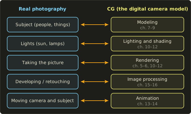
- Modeling (モデリング) builds the subject: shapes, materials, and where everything is placed.
- Lighting and shading decide where light comes from and how surfaces react to it.
- Rendering (レンダリング) is "pressing the shutter": computing the image the virtual camera sees.
- Image processing (画像処理) is the darkroom: adjusting colors, blurring, sharpening, combining images.
- Animation (アニメーション) changes the scene or the camera over time, one frame after another.
The virtual camera is a bit of a cheat, though.
It has no weight, no noise, no dust, it can be as small as a point, and it can pass through walls.
On the other hand, everything a real lens does "for free" (blur outside the focus, motion blur, lens flares) has to be computed on purpose if we want it.
To understand both sides, let's look at real cameras first.
2.2 The pinhole camera
The simplest camera there is has no lens at all.
Take a dark box, make a tiny hole in one side, and put a screen (or a sensor) on the opposite side.
Light from each point of the scene can only reach the screen through the hole, so every point of the scene lands on exactly one point of the screen.
That's the pinhole camera (ピンホールカメラ), and it's the camera model almost every CG program uses.
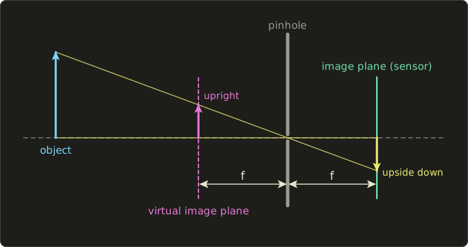
Two things to notice in the picture.
First, the image on the sensor is upside down (and mirrored left–right), because the rays cross at the hole.
Second, the distance from the hole to the image plane is called the focal length (焦点距離, shōten kyori) .
CG uses a little trick here.
If we put an imaginary screen at the same distance in front of the hole, the rays cross it at the same distances from the axis, but the image is upright.
No real camera can do that (the screen would block the light), but a virtual camera doesn't care, so CG always uses this virtual image plane.
In chapter 5 it becomes the projection plane of the perspective projection.
The formula: similar triangles
Put the pinhole at the origin and look along the axis.
A point at height and distance in front of the camera, and its image at height on the image plane at distance , form two similar triangles.
So the ratios are equal:
Far things (big ) get small, which is exactly perspective.
The Linear Algebra series, chapter 12 turned this division by into a matrix; chapter 5 of this series looks at projections from the CG point of view.
Worked example.
A person 1.7 m tall stands 10 m in front of a camera with mm.
Use millimeters everywhere: , .
The person is 8.5 mm tall on the sensor.
Walk to 5 m away and halves, so the image doubles to 17 mm.
Angle of view
How much of the scene fits in the picture depends on the sensor size and the focal length.
The angle of view (画角, gakaku), in CG usually called the field of view or FOV (視野角), is the angle between the rays that hit the two edges of the sensor:
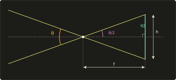
The axis cuts the picture into two right triangles with the sides and , and the angle at the pinhole.
So , and:
Worked example.
A "full-frame" sensor is 36 mm × 24 mm, and the lens has mm.
The diagonal of the sensor is mm, so the diagonal angle of view is .
Camera makers usually quote the diagonal one, while games and CG programs usually ask for the vertical or the horizontal one, so always check which one a number means.
Changing only the focal length (36 mm wide sensor):
| Focal length | Horizontal angle of view | Kind of lens |
|---|---|---|
| 24 mm | 73.7° | wide angle |
| 50 mm | 39.6° | "standard" |
| 100 mm | 20.4° | telephoto |
A shorter focal length means a wider view; a longer one zooms in.
In CG we often go the other way: we pick a field of view and an image width in pixels, and need the focal length in pixels.
Solve the formula for , with the width in pixels:
For and a horizontal FOV of 90°: , so pixels.
Why CG cameras are pinholes
A real pinhole camera is impractical: the hole lets in very little light, so exposures take seconds or minutes, and making the hole smaller to get a sharper image eventually makes things blurrier again because light bends at the edges of a tiny hole (diffraction).
A virtual pinhole has none of these problems.
It is a mathematical point, it needs no exposure time, and every point of the scene is perfectly sharp, near or far.
That's why the standard CG camera is a pinhole, and why "one ray per pixel through one point" is the heart of both rasterization (chapter 6) and ray tracing (chapter 12).
The price is that CG pictures look "too sharp".
Everything that real lenses add has to be imitated, and to imitate it we need to know what lenses do.
2.3 Real lenses and the camera's controls
A lens collects light from a big area (its opening) and bends it so that all rays from one point of the scene meet again in one point behind the lens.
That gives a much brighter image than a pinhole, but only points at one particular distance are perfectly sharp.
The thin lens equation
The simplest model of a lens is the thin lens (薄レンズ): a lens so thin that we can pretend all the bending happens in one plane.
Rays parallel to the axis are bent through the focal point at distance behind the lens, rays through the center go straight on, and rays through the front focal point leave the lens parallel to the axis:
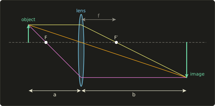
If the object is at distance in front of the lens and its sharp image forms at distance behind it, the thin lens equation (レンズの公式) says:
The picture is drawn with , , (any unit): .
The image is times as big as the object and upside down, just like in the pinhole camera.
Worked example.
A 50 mm lens is focused on a subject 2 m (2000 mm) away.
How far behind the lens must the sensor be?
For a subject at 1 m, the same calculation gives mm.
That's what focusing is: moving the lens a millimeter or two away from the sensor.
And when the subject is very far away, goes to 0 and .
That's the real definition of focal length: the lens-to-sensor distance when focused at infinity.
The magnification is , so a 1.7 m person 2 m away is mm tall on the sensor (too tall for a 24 mm sensor, so only the upper body fits).
The pinhole formula would give mm: the two models agree better and better as the subject gets further away, because approaches .
Aperture and f-number
Inside the lens is an adjustable hole, the aperture (絞り, shibori), with diameter .
Its size is given as the f-number (F値):
A 50 mm lens at f/2 has an opening of mm; at f/8 it's mm.
So a bigger f-number means a smaller hole, which trips up almost everybody at first.
The light that gets through is proportional to the area of the hole, so to , and therefore to .
That's why the standard f-numbers go 1.4, 2, 2.8, 4, 5.6, 8, 11, 16: each one is about times the previous one, which halves the area and halves the light.
One such step is called a stop.
Depth of field and the circle of confusion
When the lens is focused at distance , a point at another distance doesn't converge on the sensor.
Its light cone is cut by the sensor before or after its tip, and makes a small disc instead of a point: the circle of confusion (錯乱円, sakuran'en).
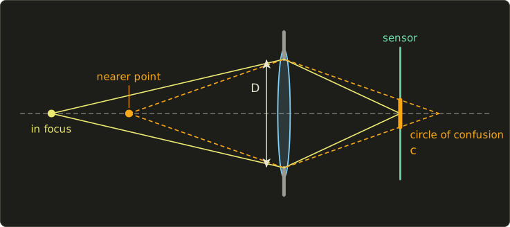
From similar triangles in this picture (using the thin lens equation for both points) the diameter of that disc is:
If is smaller than what we can notice in the final picture, the point still looks sharp.
The range of distances that look sharp is the depth of field (被写界深度, hishakai shindo).
Worked example.
A 50 mm lens at f/2 ( mm) is focused at mm.
How big is the blur of a point at mm?
For a full-frame sensor, about 0.03 mm is the usual limit for "looks sharp", so this background point is a disc more than ten times too big: clearly blurred.
You don't need the exact depth of field formula, but you should know the trends.
For subjects that aren't too far away, a good approximation of the total depth of field is:
With , mm, mm, mm:
Only about 19 cm around the subject is sharp.
At f/8 the same formula gives mm.
(The exact values, which I computed with the full formulas, are about 188 mm and 776 mm, so the approximation is good here.)
Reading the formula:
- A bigger f-number (smaller aperture) gives a deeper depth of field. A pinhole is the extreme case: everything is sharp.
- A longer focal length gives a shallower depth of field ( is in the denominator).
- A closer subject gives a shallower depth of field ( in the numerator).
In CG, the depth-of-field effect (被写界深度効果) is made either physically, by replacing the pinhole with a thin lens and shooting rays from random points of the aperture, or cheaply, by blurring each pixel of a finished image by its own circle of confusion computed from its depth.
Games mostly do the second; film renderers mostly the first.
Shutter speed and motion blur
The shutter (シャッター) decides how long the sensor collects light: the shutter speed or exposure time , like 1/60 s or 1/1000 s.
Anything that moves during that time is smeared along its path: motion blur (モーションブラー).
Worked example.
A car crosses the image at 1200 pixels per second, and the shutter is open for 1/60 s.
It moves pixels while the shutter is open, so it's smeared over 20 pixels.
At 1/1000 s it would move only 1.2 pixels and look frozen.
Film traditionally runs at 24 frames per second with the shutter open for half of each frame (1/48 s), so movies contain a lot of motion blur, and our eyes expect it.
A CG camera has an exposure time of zero unless we say otherwise: every frame is a perfectly frozen instant.
To add motion blur, a renderer averages the scene over several moments within the "shutter time", or blurs pixels along their motion in a post-process.
We'll see in sections 2.6 and 2.7 that this is really a form of anti-aliasing in time.
Exposure
How bright the picture comes out is the exposure (露出).
Three controls set it:
- the aperture: light is proportional to ,
- the shutter speed: light is proportional to ,
- the sensitivity (感度, the ISO value): doubling it doubles the signal, but also amplifies the noise.
Photographers combine aperture and shutter into one number, the exposure value:
f/8 at 1/125 s gives , so about EV 13.
f/5.6 at 1/250 s gives , also about EV 13.
One stop more light from the aperture, one stop less from the shutter: the same exposure, but a shallower depth of field and less motion blur.
Every exposure choice is a trade between brightness, depth of field, motion blur and noise.
In CG, "exposure" is just a number we multiply the computed light by before turning it into displayable pixel values (tone mapping, chapter 15), but physically based renderers often let you type in real f-numbers, shutter speeds and ISO values so the results match real photography.
Lens distortion and vignetting
Real lenses aren't perfect.
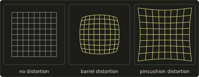
The most visible flaw is distortion (歪曲収差): straight lines near the edge of the picture bend.
A simple model moves every point along its distance from the image center:
With the corners are pulled in (barrel distortion, 樽型), typical of wide-angle lenses; with they're pushed out (pincushion distortion, 糸巻き型), typical of telephoto lenses.
These grids were computed with exactly that formula ( and ):
Other imperfections you'll meet:
- Vignetting (周辺減光, shūhen genkō): the corners are darker than the center. Even an ideal lens has natural vignetting that falls off roughly with of the angle from the axis.
- Chromatic aberration (色収差): glass bends different wavelengths by different amounts, so edges get thin colored fringes.
- Lens flare: bright lights reflect inside the lens and leave rings and streaks.
CG imitates all of these as post-effects on the finished image, because a perfect virtual camera looks artificial.
In the opposite direction, computer vision calibrates real cameras (measures and friends) to remove distortion, so photos can be combined with CG precisely (chapter 14).
Try it in code (optional)
A few lines of C++ that compute the numbers of this section, so you can try your own lenses:
#include <cmath>
#include <cstdio>
#include <numbers>

// Angle of view (radians) of a sensor of size h behind a pinhole/lens of focal length f
double angleOfView(double h, double f) {
  return 2.0 * std::atan(h / (2.0 * f));
}

// Thin lens: image distance b for an object at distance a (1/f = 1/a + 1/b)
double imageDistance(double f, double a) {
  return 1.0 / (1.0 / f - 1.0 / a);
}

// Diameter of the circle of confusion for a point at distance a,
// when a lens with focal length f and aperture D is focused at distance af
double circleOfConfusion(double f, double D, double af, double a) {
  return D * f * std::fabs(a - af) / (a * (af - f));
}

double degrees(double rad) { return rad * 180.0 / std::numbers::pi; }

int main() {
  double f = 50.0;  // mm
  printf("horizontal: %.1f deg\n", degrees(angleOfView(36.0, f)));
  printf("vertical:   %.1f deg\n", degrees(angleOfView(24.0, f)));
  printf("diagonal:   %.1f deg\n", degrees(angleOfView(std::hypot(36.0, 24.0), f)));
  printf("b = %.2f mm\n", imageDistance(f, 2000.0));
  double N = 2.0;   // f-number
  double D = f / N; // aperture diameter
  printf("c = %.3f mm\n", circleOfConfusion(f, D, 2000.0, 4000.0));
  long bytes = 1920L * 1080L * 3L;
  printf("1920x1080 RGB: %ld bytes (%.2f MiB)\n", bytes, bytes / (1024.0 * 1024.0));
}
horizontal: 39.6 deg
vertical:   27.0 deg
diagonal:   46.8 deg
b = 51.28 mm
c = 0.321 mm
1920x1080 RGB: 6220800 bytes (5.93 MiB)
The last line is a preview of section 2.5.
2.4 The image sensor
Behind the lens of a digital camera sits the image sensor (撮像素子, satsuzō soshi), a chip covered with millions of tiny light-sensitive cells called photosites.
Each photosite turns the light (photons) that falls on it during the exposure into electric charge, the charge becomes a voltage, and an analog-to-digital converter turns the voltage into an integer, typically with 12 or 14 bits.
That's the moment the picture becomes numbers.
(Today's sensors are almost all CMOS sensors; the older CCD type works on the same principle.)
A photosite only measures how much light arrived, not its color.
To get color, almost every camera puts a tiny color filter on top of each photosite, in a repeating pattern called a color filter array.
The most common one is the Bayer filter (ベイヤー配列), patented by Bryce Bayer at Kodak in 1976:
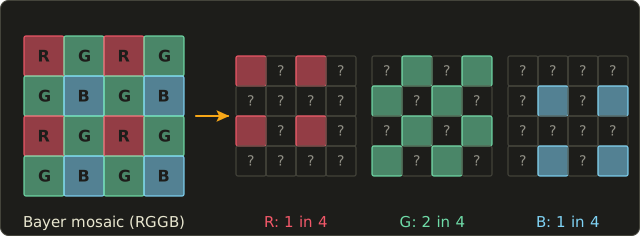
Half of the photosites are green, a quarter red and a quarter blue.
Green gets twice as many because our eyes get most of their sense of brightness and detail from the green part of the spectrum (chapter 3).
So the raw sensor data is a mosaic, and every pixel knows only one of its three colors.
The two missing ones are estimated from the neighbors: that's demosaicing (デモザイク).
The simplest method is averaging.
At a red photosite, the four direct neighbors are green, so if they measured 100, 104, 96 and 108:
Real cameras use much smarter methods that follow edges, because simple averaging makes colored fringes along sharp edges.
After demosaicing, the camera adjusts white balance and colors, compresses the result (often to JPEG, section 2.10), and you get the familiar RGB image.
A renderer has none of this: it computes red, green and blue for every pixel directly.
But it's worth knowing, because "realistic" CG often adds the sensor's typical flaws back: noise, film grain, and rolling shutter distortion (many CMOS sensors read the rows one after another, so fast-moving things lean).
2.5 Digital images: sampling and quantization
Now to the picture itself.
The light falling on the sensor is a continuous image: brightness and color are defined at every point, and can take any value.
A computer can only store finitely many numbers, so two things must be made discrete:
- where we measure, and
- what values we can store.
The first step is sampling (標本化, hyōhonka): we keep the value only at regular positions.
The second is quantization (量子化, ryōshika): we round each kept value to one of a fixed number of levels.
Here's the same idea in one dimension, with a curve sampled at 13 positions and then quantized to 8 levels:
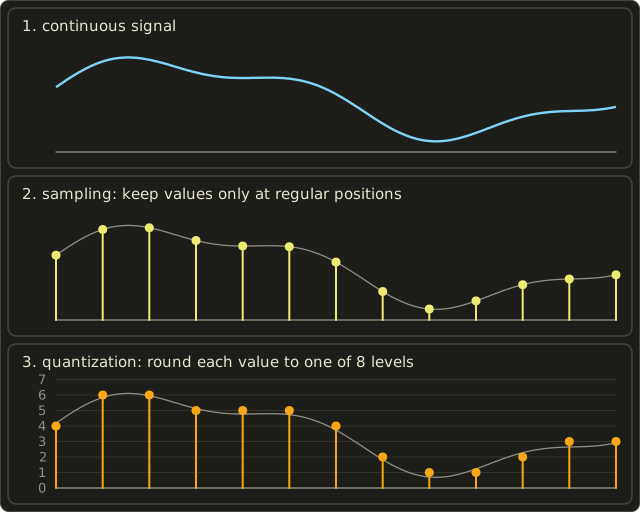
An image is the same in two dimensions: sampled on a grid in x and y, and quantized in value.
The result is a digital image (ディジタル画像): a rectangular array of numbers.
Video adds a third sampling direction, time: 24, 30 or 60 frames per second.
Pixels, resolution and aspect ratio
Each sample of a digital image is a pixel (画素, gaso; short for "picture element").
It's tempting to think of a pixel as a little colored square, and that's how screens show them, but mathematically a pixel is a sample of the continuous image at one point.
Keeping that in mind makes the rest of this chapter much easier.
Image coordinates usually start at the top-left corner with y pointing down, the opposite of math (chapter 4 deals with that).
Resolution (解像度, kaizōdo) has two meanings, and both are worth knowing for the exam:
- the number of pixels, like 1920 × 1080 (width × height), and
- the density of pixels, like 300 dpi (dots per inch) for print or the ppi (pixels per inch) of a screen.
1920 × 1080 is pixels, about 2.1 megapixels.
Printed at 300 dpi it becomes inches by inches, which is about 16.3 cm × 9.1 cm: the same pixels, a fixed physical size.
The aspect ratio (アスペクト比) is width : height.
The greatest common divisor of 1920 and 1080 is 120, and , , so 1920 × 1080 is 16:9.
640 × 480 is 4:3, the old TV shape.
Bit depth and number of levels
Quantization is described by the bit depth (ビット深度): how many bits store one value.
With bits we get levels, the number of gray levels or gradations (階調数, kaichōsū):
| Bits per channel | Levels | Typical use |
|---|---|---|
| 1 | 2 | black and white only (fax, simple printers) |
| 8 | 256 | normal images and screens |
| 10 | 1024 | HDR video, wide-gamut displays |
| 16 | 65,536 | photo editing, scientific images |
A grayscale image (グレースケール, 濃淡画像) has one value per pixel, its brightness.
A color image usually has three values per pixel, red, green and blue: three channels (チャンネル).
With 8 bits per channel, that's 24 bits per pixel and
possible colors, often called full color or "true color" (フルカラー).
A fourth channel, alpha (アルファ), often stores how opaque each pixel is (0 = fully transparent, 1 = fully opaque); we'll need it for compositing in chapter 14.
How big is an image?
Pixels times channels times bytes per channel.
A 1920 × 1080 RGB image with 8 bits per channel:
That's about 6.2 MB, or MiB.
With alpha (RGBA) it's bytes.
And uncompressed video at 60 frames per second would need bytes, about 373 MB, every second.
That's why compression (section 2.10) isn't optional.
Quantization in numbers
Let's write values as numbers from 0 (black) to 1 (white).
With levels, the stored integer and the value it stands for are:
The steps are apart, so the error is never more than half a step, .
Worked example.
Store with 3 bits ( levels):
The error is , well below the maximum .
With 8 bits () the steps are only apart, so the error is at most about 0.002.
2.6 The sampling theorem and aliasing
Sampling throws away everything between the samples.
When is that harmless?
The answer is the most important formula of this chapter.
Frequencies and the sampling theorem
Any signal, including a row of an image, can be described as a sum of waves of different frequencies.
Slow changes (a smooth sky) are low frequencies; fast changes (fine stripes, sharp edges, text) are high frequencies.
The sampling theorem (標本化定理, hyōhonka teiri; also called the Nyquist–Shannon theorem) says:
A signal whose highest frequency is can be reconstructed exactly from its samples if the sampling frequency is more than twice that frequency.
Half of the sampling frequency, , is the highest frequency we can represent: the Nyquist frequency (ナイキスト周波数).
Worked example.
Humans hear up to about 20 kHz.
Audio CDs sample at 44.1 kHz, so their Nyquist frequency is kHz, just above what we can hear.
For an image, the sampling frequency is 1 sample per pixel, so the Nyquist frequency is 0.5 cycles per pixel: one cycle every 2 pixels.
The finest pattern an image can hold is alternating black and white pixels; anything finer than that can't be stored.
Aliasing
What happens if we sample a frequency above the Nyquist frequency anyway?
It doesn't just disappear.
It shows up disguised as a lower frequency, like a person using someone else's name.
That's aliasing (エイリアシング), and the false frequency is called an alias.
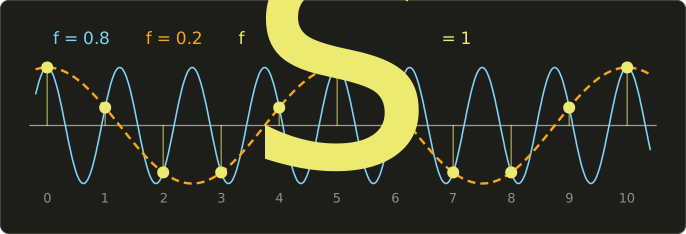
The blue wave makes 0.8 cycles per sample, far above the Nyquist frequency 0.5.
The yellow samples are all we keep, and they lie exactly on the orange wave with only 0.2 cycles per sample.
From the samples alone, nobody can tell the two apart.
In general, a frequency sampled at looks like for the whole number that brings it below .
Here: .
We can check one sample: at , and .
In images and animation, aliasing has three famous faces.
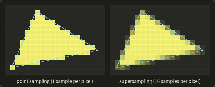
Jaggies (ジャギー): a slanted edge contains arbitrarily high frequencies (it's a sudden jump).
Sampling it with one sample per pixel turns the smooth line into a staircase:
Moiré (モアレ): a fine regular pattern sampled too coarsely turns into big, wrong patterns.
The left picture is a "zone plate", rings that get finer towards the edge.
In the middle it is sampled at 48 × 48 pixels with one sample per pixel: wherever the rings are finer than 2 pixels, completely new rings appear that aren't in the original.
On the right, each pixel averages 8 × 8 samples instead (section 2.7): the too-fine rings become a mostly flat gray, which is the honest answer.
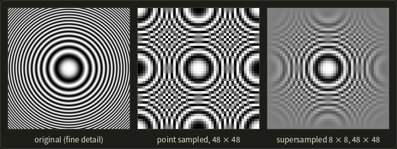
You've seen moiré on photos of TV screens, striped shirts and fences, and in games as the shimmering of distant fences and floor tiles.
Temporal aliasing (時間方向のエイリアシング): frames are samples in time, so fast motion aliases too.
The classic case is the wagon-wheel effect: in films, wheels sometimes seem to stand still or turn backwards.
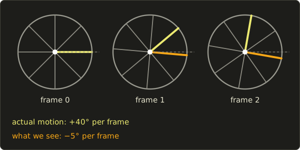
Worked example.
A wheel with 8 identical spokes looks the same every .
At 24 frames per second it turns per frame (that's , or 2.67 turns, per second).
After one frame, the spoke that is now closest to where a spoke was before is the one at .
Our eyes match nearest spokes, so we see the wheel turning backwards by per frame, per second.
2.7 Anti-aliasing
Techniques that reduce aliasing are called anti-aliasing (アンチエイリアシング).
The sampling theorem tells us there are only two honest ways:
- remove the frequencies that are too high before sampling, so there is nothing left to alias, or
- sample more often, which raises the Nyquist frequency.
Real cameras do the first in hardware: many sensors have an optical low-pass filter in front of them that slightly blurs the image before the photosites sample it, exactly to prevent moiré.
CG has to do it in software.
Point sampling, area sampling and supersampling
Take one pixel crossed by the edge of a yellow shape that covers the lower-left part of the pixel.
Here's what three methods compute for it:
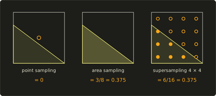
- Point sampling looks only at the pixel center. The center is outside the shape, so the pixel gets 0% of the shape's color. A tiny shift of the edge would flip it to 100%: that's where jaggies come from.
- Area sampling (エリアサンプリング) uses the fraction of the pixel's area that the shape covers. The covered part is a triangle with legs 1 and 0.75, so its area is .
- Supersampling (スーパーサンプリング) takes many samples inside the pixel and averages them. With a 4 × 4 grid, 6 of the 16 samples are inside: .
If the shape is white on black, the pixel becomes , and in 8 bits : a dark gray that makes the edge look smooth from a normal viewing distance.
In terms of filtering, area sampling is pre-filtering (プリフィルタリング): the continuous image is averaged (low-pass filtered) over the pixel's area before we take one sample per pixel.
Supersampling is post-filtering (ポストフィルタリング): we first sample at a higher rate, and afterwards filter (average) the samples down to one value per pixel.
Averaging with equal weights is the simplest filter, the box filter; renderers often use smoother ones (tent, Gaussian) that also give some weight to samples in neighboring pixels.
The price of supersampling is speed.
4 × 4 samples per pixel means 16 times the work: for 1920 × 1080 that's samples per frame.
That's why GPUs use cheaper variants like MSAA (it's introduced with the drawing pipeline in chapter 6 and deepened in Part 2; you'll turn it on yourself in OpenGL chapter 20).
Games also use post-process anti-aliasing, which looks for staircase edges in the finished image and smooths them.
That's cheap, but it can't bring back detail that sampling already lost (it can't fix the moiré in the middle picture above).
Anti-aliasing in time
The same two ideas work in time.
Pre-filtering in time means averaging over the shutter interval: that's exactly motion blur.
A wheel rendered with proper motion blur turns into a blurred disc instead of turning backwards.
That's one reason film's 24 frames per second look smooth, while a game at 24 frames per second without motion blur looks choppy.
2.8 Quantization effects: false contours and dithering
Too few levels cause their own artifact.
A smooth gradient becomes a staircase of flat bands, and the steps between the bands look like edges that aren't in the scene.
These are false contours (疑似輪郭, giji rinkaku), also called banding.
Here is the same shaded sphere quantized to 2, 4, 8 and 256 levels:
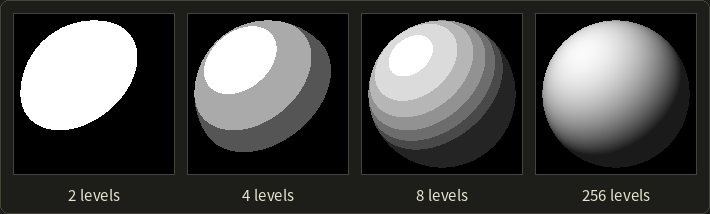
With 8 levels the sphere looks like a contour map.
With 256 levels it looks smooth, at least here.
But stretch 256 levels across a 1920-pixel-wide gradient and each level becomes a band pixels wide.
In dark, smooth areas (night skies, fog, shadows) those bands can become visible, because our vision exaggerates the edges between flat areas (lateral inhibition, the effect behind the Mach bands of chapter 3).
That's one reason HDR video uses 10 bits.
Dithering
If we can't add levels, we can trade spatial resolution for them.
Dithering (ディザリング) adds a pattern or noise before quantizing, so that the average over a small area has the right brightness even if each pixel is only black or white:
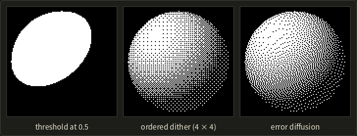
- Ordered dithering (組織的ディザ法) compares each pixel with a threshold from a small repeating matrix. With the 4 × 4 Bayer matrix (no relation to the sensor; same family name), the 16 thresholds are for . A flat gray of 0.3 is above the thresholds for (because but ), so 5 of every 16 pixels turn white: an average of .
- Error diffusion (誤差拡散法), for example the Floyd–Steinberg method, rounds each pixel and pushes its rounding error onto the neighbors that haven't been processed yet (with the weights 7/16, 3/16, 5/16 and 1/16), so errors cancel out over an area.
Dithering is still everywhere: printers (which only have ink or no ink), GIF images, and high-quality rendering, where a tiny bit of noise before converting to 8 bits hides banding in skies and fog.
Here it is as a shader function that reduces a color to levels levels per channel, with or without an ordered dither:
static const float bayer4[16] = { 0.0, 8.0, 2.0, 10.0, 12.0, 4.0, 14.0, 6.0,
                                  3.0, 11.0, 1.0, 9.0, 15.0, 7.0, 13.0, 5.0 };

// Round c to `levels` levels per channel. With dither, add an ordered-dither offset first.
float3 quantize(float3 c, float levels, uint2 pixel, bool dither) {
  float offset = 0.0;
  if (dither) {
    offset = (bayer4[(pixel.y % 4) * 4 + (pixel.x % 4)] + 0.5) / 16.0 - 0.5;
  }
  return round(c * (levels - 1.0) + offset) / (levels - 1.0);
}
const float bayer4[16] = float[16](0.0, 8.0, 2.0, 10.0, 12.0, 4.0, 14.0, 6.0,
3.0, 11.0, 1.0, 9.0, 15.0, 7.0, 13.0, 5.0);
// Round c to `levels` levels per channel. With dither, add an ordered-dither offset first.
vec3 quantize(vec3 c, float levels, uvec2 pixel, bool dither) {
float offset = 0.0;
if (dither) {
offset = (bayer4[(pixel.y % 4u) * 4u + (pixel.x % 4u)] + 0.5) / 16.0 - 0.5;
}
return round(c * (levels - 1.0) + offset) / (levels - 1.0);
}static const float bayer4[16] = { 0.0, 8.0, 2.0, 10.0, 12.0, 4.0, 14.0, 6.0,
3.0, 11.0, 1.0, 9.0, 15.0, 7.0, 13.0, 5.0 };
// Round c to `levels` levels per channel. With dither, add an ordered-dither offset first.
float3 quantize(float3 c, float levels, uint2 pixel, bool dither) {
float offset = 0.0;
if (dither) {
offset = (bayer4[(pixel.y % 4) * 4 + (pixel.x % 4)] + 0.5) / 16.0 - 0.5;
}
return round(c * (levels - 1.0) + offset) / (levels - 1.0);
}The offset is always between −0.5 and +0.5 of a step, so the result stays between 0 and 1, and over a 4 × 4 tile the rounding errors average out.
2.9 Raster images and vector images
Everything so far was about raster images (ラスタ画像): grids of pixels.
There's a second way to store a picture: describe the shapes and let the computer draw them when needed.
That's a vector image (ベクタ画像).
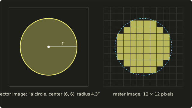
The vector circle on the left is stored as three numbers (center x, center y, radius) and a color.
The raster circle on the right is 144 pixels, and each one is either inside or outside: the pixels whose centers lie inside the circle.
| Raster image | Vector image | |
|---|---|---|
| Stores | pixel values | shapes: points, lines, curves, fills |
| Scaling up | gets blocky or blurry | stays sharp at any size |
| Good for | photos, rendered images, textures | logos, fonts, diagrams, UI, CAD drawings |
| Formats | PNG, JPEG, GIF, BMP, TIFF, WebP, EXR | SVG, PDF, EPS |
Every diagram in this series is a vector image (SVG), and the fonts you're reading are vector outlines made of curves (chapter 8 covers the curves).
A screen can only show pixels, though, so a vector image must always be turned into a raster image in the end.
That conversion is rasterization or scan conversion (ラスタライズ/スキャン変換), and it's exactly what a GPU does with triangles (chapter 6).
3D CG is vector graphics in 3D: the models are shapes, and the image is their rasterization.
2.10 Image file formats and compression
We saw that one Full HD frame is about 6 MB.
Compression makes it smaller, in one of two ways:
- Lossless compression (可逆圧縮): the file is smaller, but decompressing gives back exactly the original pixels.
- Lossy compression (非可逆圧縮): some information is thrown away for good, ideally the part we wouldn't notice anyway. Files get much smaller.
A tiny lossless example is run-length encoding: the row WWWWWWBBBWWWW (13 pixels) can be stored as "6 W, 3 B, 4 W".
It's 6 symbols instead of 13, and decoding gives back exactly the same row.
Real formats use cleverer schemes, but the idea is the same: describe repetition instead of storing it.
| Format | Compression | Notes |
|---|---|---|
| BMP | usually none | simple, big files |
| PNG | lossless | up to 16 bits per channel, alpha; screenshots, UI, textures with sharp edges |
| GIF | lossless, but at most 256 colors | palette images, simple animations |
| JPEG | lossy | photos; no alpha |
| WebP, AVIF | lossy or lossless | newer web formats with better compression |
| TIFF | usually lossless | print and scanning, many bits per channel |
| OpenEXR, Radiance HDR | lossless or lossy, floating point | HDR images for film and rendering |
Note the trap in GIF: the compression itself is lossless, but a full-color photo first has to be reduced to 256 colors, and that loses information.
What JPEG throws away
JPEG is worth understanding, because it's built on ideas from this chapter:
- It converts RGB to YCbCr: one brightness channel Y and two color-difference channels Cb and Cr (chapter 3 has the formulas).
- Our eyes see fine detail mostly in brightness, not in color. So the color channels are stored at lower resolution: chroma subsampling (クロマサブサンプリング). The common 4:2:0 mode keeps one Cb and one Cr value per 2 × 2 pixels, which alone halves the data (chapter 3 works out the numbers and the other modes).
- Each channel is cut into 8 × 8 blocks, and each block is rewritten as a sum of 64 cosine patterns with the DCT (discrete cosine transform, 離散コサイン変換).
- The amounts of each pattern are quantized: coarsely for high frequencies, finely for low ones. Many high-frequency amounts become 0. This is where the real loss happens, and the "quality" setting controls how coarse it is.
- The many zeros compress very well with ordinary lossless coding.
These are the 64 patterns, from flat (top left) to the finest checkerboard (bottom right):
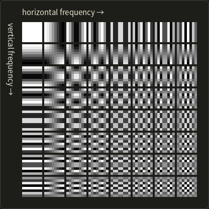
The typical JPEG artifacts follow directly: visible 8 × 8 blocks at low quality, ringing (faint ripples, "mosquito noise") next to sharp edges where high frequencies were cut, and smeared colors at sharp color edges.
That's why text, UI, pixel art and normal maps should not be stored as JPEG.
A teaser: HDR images
In everyday use, the formats above (except the last row) store values from 0 to 1, in other words "as bright as the screen can show".
The real world has a far larger range: the sun is many thousands of times brighter than a shadow.
HDR images (high dynamic range, ハイダイナミックレンジ画像) store real light values as floating-point numbers, for example in OpenEXR (16- or 32-bit floats per channel).
Renderers work in HDR internally, and the step that maps HDR down to what a screen can show is tone mapping.
We'll come back to HDR in chapter 15 and in Part 2.
2.11 CG and image processing
Last, the third syllabus item: how CG relates to its neighbors.
We already met the rule in chapter 1: tell the three fields apart by what goes in and what comes out.
CG is model → image (that's the digital camera model), image processing (画像処理) is image → image (chapter 15), and computer vision (コンピュータビジョン) together with image recognition (画像認識) is image → model or description.
Because vision runs CG backwards, it's sometimes called "inverse graphics".
In real work they constantly meet:
- Textures from photos: photographs of real surfaces, processed to tile seamlessly, are mapped onto models (chapter 11).
- Image-based rendering (イメージベーストレンダリング): new views are computed directly from photos instead of from 3D models, and HDR photos of real places are used as the light of CG scenes (rendering chapters 11 and 12).
- Compositing (合成): CG is combined with live-action film. Computer vision tracks the real camera's motion from the footage ("match moving"), so the CG camera can copy it exactly, and image processing blends the layers (chapter 14).
- 3D scanning and photogrammetry: a model is reconstructed from many photos or a scanner, then rendered (chapter 17).
- Motion capture: cameras track markers on an actor, and the motion drives a CG character (chapter 13).
- Post-processing in games: bloom, depth of field, motion blur, tone mapping and anti-aliasing are image processing applied to the rendered frame, every frame.
- Computational photography: smartphones combine many photos into one (HDR merging, night modes, background blur) using all three fields at once (chapter 16).
So the boundary isn't a wall.
For the exam, remember the in/out rule; for practice, remember that modern pipelines use all three.
Exam points
The distinctions worth being sure about:
- Sampling (標本化) makes the positions discrete (where we measure); quantization (量子化) makes the values discrete (how finely we store them). Resolution belongs to sampling, the number of levels (階調数) and bit depth to quantization.
- Too coarse sampling causes aliasing (jaggies, moiré, the wagon-wheel effect). Too few levels cause false contours (疑似輪郭). Don't mix them up.
- The sampling theorem: sample at more than twice the highest frequency. The Nyquist frequency is half the sampling frequency.
- bits give levels: 8 bits → 256, 24-bit color → 16,777,216 colors. Image size = width × height × channels × bytes per channel.
- Anti-aliasing: area sampling = pre-filtering (filter, then sample); supersampling = post-filtering (sample densely, then filter). Motion blur is anti-aliasing in time.
- : a bigger f-number is a smaller aperture, less light, and a deeper depth of field. A pinhole camera has everything in focus.
- Thin lens: ; focused at infinity, . Angle of view: ; longer focal length → narrower view.
- PNG and GIF are lossless (GIF limited to 256 colors), JPEG is lossy (YCbCr, chroma subsampling, 8 × 8 DCT, quantization).
- CG: model → image; image processing: image → image; computer vision / image recognition: image → model or description.
2.12 Summary
- CG can be seen as a digital camera model: modeling, lighting, rendering, image processing and animation correspond to subject, lights, shooting, developing and moving the camera.
- The pinhole camera projects every scene point through one point: . Its image is upside down; CG uses a virtual image plane in front of the pinhole. Angle of view .
- Real lenses follow . The f-number , shutter speed and sensitivity set the exposure and bring depth of field (circle of confusion), motion blur and noise. Lenses also distort and vignette; CG imitates all of this on purpose.
- A sensor measures light with photosites behind a Bayer filter; demosaicing fills in the missing colors.
- A digital image is a continuous image after sampling (positions → pixels, resolution) and quantization (values → levels). Size = width × height × channels × bytes.
- The sampling theorem demands . Violating it causes aliasing: jaggies, moiré, wagon wheels. Anti-aliasing pre-filters (area sampling) or samples more and post-filters (supersampling); motion blur does it in time.
- Too few levels cause false contours; dithering trades resolution for apparent levels.
- Raster images store pixels, vector images store shapes and must be rasterized to be shown.
- Lossless (PNG) vs lossy (JPEG) compression; JPEG removes color detail and high frequencies. HDR images store real light values.
- CG (model → image), image processing (image → image) and computer vision (image → model) meet in textures, image-based rendering, compositing, scanning and post-processing.
2.13 Key terms
| English | 日本語 |
|---|---|
| digital camera model | ディジタルカメラモデル |
| pinhole camera | ピンホールカメラ |
| focal length | 焦点距離 |
| angle of view / field of view | 画角/視野角 |
| thin lens | 薄レンズ |
| aperture | 絞り |
| f-number | F値 |
| depth of field | 被写界深度 |
| circle of confusion | 錯乱円 |
| shutter speed | シャッター速度 |
| motion blur | モーションブラー |
| exposure | 露出 |
| lens distortion (barrel, pincushion) | 歪曲収差(樽型、糸巻き型) |
| vignetting | 周辺減光 |
| image sensor | 撮像素子 |
| Bayer filter | ベイヤー配列 |
| demosaicing | デモザイク |
| digital image | ディジタル画像 |
| sampling | 標本化 |
| quantization | 量子化 |
| pixel | 画素(ピクセル) |
| resolution | 解像度 |
| aspect ratio | アスペクト比 |
| bit depth | ビット深度 |
| number of gray levels | 階調数 |
| grayscale image | 濃淡画像(グレースケール画像) |
| channel / alpha | チャンネル/アルファ |
| sampling theorem | 標本化定理 |
| Nyquist frequency | ナイキスト周波数 |
| aliasing | エイリアシング |
| jaggies | ジャギー |
| moiré | モアレ |
| anti-aliasing | アンチエイリアシング |
| supersampling | スーパーサンプリング |
| area sampling | エリアサンプリング |
| false contour | 疑似輪郭 |
| dithering | ディザリング |
| raster image / vector image | ラスタ画像/ベクタ画像 |
| lossless / lossy compression | 可逆圧縮/非可逆圧縮 |
| image processing | 画像処理 |
| computer vision / image recognition | コンピュータビジョン/画像認識 |
| image-based rendering | イメージベーストレンダリング |
2.14 Challenges
- ★ A camera has a 36 mm wide sensor and a 35 mm lens. Compute the horizontal angle of view in degrees (one decimal).
- ★ A thin lens with mm is focused on a subject 3 m away. How far behind the lens is the sensor, and what is the magnification ?
- ★ How many bytes does an uncompressed 3840 × 2160 RGBA image with 8 bits per channel need, and how many bytes are 10 seconds of such frames at 30 frames per second?
- ★ Quantize the values 0.1, 0.45 and 0.8 to 4 levels (2 bits) with , and give the error of each; check that none exceeds half a step.
- ★★ A striped pattern repeats every 1.6 pixels and is point-sampled once per pixel. Which frequency (in cycles per pixel) appears in the image, and how many pixels long is one period of that alias?
- ★★ A wheel with 8 identical spokes is filmed at 24 frames per second. At which rotation speeds (in turns per second) does it seem to stand still? Give the three slowest.
- ★★★ Explain why a pinhole CG camera never shows depth of field, what you would have to add to the renderer to get it, and why making the hole of a real pinhole camera ever smaller does not make its images ever sharper.
Multiple choice
Q1 ★ Which of the following correctly describes quantization of a digital image?
| A | Choosing the positions at which the continuous image is measured |
| B | Estimating the missing colors of each photosite from its neighbors |
| C | Reducing the file size by removing high frequencies |
| D | Rounding each measured value to one of a finite number of levels |
| E | Averaging several samples inside each pixel |
Q2 ★★ An audio signal contains frequencies up to 15 kHz. Which sampling frequency allows it to be reconstructed without aliasing?
| A | 40 kHz |
| B | 25 kHz |
| C | 20 kHz |
| D | 15 kHz |
| E | 10 kHz |
Q3 ★★ Which change makes the depth of field of a camera deeper, if everything else stays the same?
| A | Opening the aperture (a smaller f-number) |
| B | Switching to a lens with a longer focal length |
| C | Using a longer shutter time |
| D | Using a higher ISO sensitivity at the same aperture |
| E | Stopping down the aperture (a larger f-number) |
2.15 Practical assignment
Be the camera.
In this assignment you'll take one "picture" completely by hand: design a camera, sample a shape, anti-alias it, quantize it and compute the file size.
You need graph paper (5 mm squares are ideal), a ruler, a protractor, a pencil and a calculator.
Part A: the camera.
- Step 1: For a 36 mm wide sensor, compute the horizontal angle of view for , 50 and 100 mm with .
- Step 2: Draw each camera to scale from the side (1 mm = 1 mm, or 2 mm per graph square): a point for the pinhole, a 36 mm line for the sensor at distance , and the two edge rays through the pinhole, extended to the other side.
- Step 3: Measure the angle between the rays with the protractor.
Check: your measured angles should agree with your computed ones to within about 1°, and the order must be "shorter focal length, wider angle".
Part B: sampling and anti-aliasing.
- Step 4: Draw an 8 × 8 pixel grid with each pixel 4 × 4 squares (so 32 × 32 squares in total). Use pixel units with the origin at the top-left corner and y pointing down.
- Step 5: Draw the triangle with corners , and (in pixels) with a sharp pencil and a ruler.
- Step 6: Point sampling: mark the center of every pixel, and color the pixels whose center is inside the triangle. Count them.
- Step 7: Supersampling: in every pixel, check the centers of its 16 small squares (a 4 × 4 grid of samples) and write the number inside the triangle (0 to 16) into the pixel.
- Step 8: Compute the triangle's exact area with the shoelace formula .
Check: the sum of all your counts divided by 16 is the supersampled estimate of the area. For this triangle it should come out exactly equal to the area from step 8 (no sample lies exactly on an edge). If you're off, recheck the pixels along the edges.
Then compare your point-sampled picture and your counts: where does the point-sampled picture have staircases, and how do the counts soften them?
Part C: quantization and size.
- Step 9: Quantize every pixel's coverage to 4 levels (2 bits) with , and shade the pixels with 4 pencil tones (0 = white, 3 = darkest).
- Step 10: Compute how many bytes your image needs at 2 bits per pixel, and how many it would need as a 24-bit color image.
Check: every fully covered pixel (count 16) must become level 3, every empty one level 0, and the 2-bit image must be exactly 1/12 the size of the 24-bit one.
Finally, hold the paper at arm's length and compare the point-sampled triangle with the 4-level one: that's anti-aliasing working on your own eyes.
コメント(0)
まだコメントはありません。
ログインするとコメント出来ます。