6. Matrices and Matrix–Vector Multiplication
So far we've worked with vectors: arrows and lists of numbers.
In this chapter we meet the other main character of linear algebra, the matrix.
A matrix is the thing that takes a vector and turns it into a different vector.
Every vertex of every model you've ever seen in a game went through at least one matrix before it reached the screen, usually several, every single frame.
The good news is that you already know everything you need.
Multiplying a matrix by a vector is nothing more than the dot products from chapter 4, or, looked at another way, the linear combinations of basis vectors from chapter 2.
By the end of this chapter you'll see why those two ideas are the same thing, and you'll be able to read any matrix and tell what it does just by looking at its columns.
6.1 What is a matrix?
A matrix is a rectangular grid of numbers.
That's really all it is.
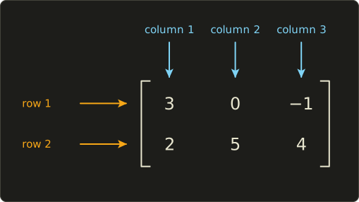
Here is one:
The horizontal lines of numbers are called rows, and the vertical lines are called columns.
This matrix has 2 rows and 3 columns, so we call it a 2 × 3 matrix (read "two by three").
In general a matrix with rows and columns is an m × n matrix.
The order is always rows first, then columns.
I remember it as "RC", like a remote-control car.
We write matrices with bold uppercase letters like or , just as vectors get bold lowercase letters like .
Elements and the m-i-j notation
Each number inside a matrix is called an element (or entry).
To point at one element, we give its row number and its column number, in that order, as a small subscript.
For the matrix we use the lowercase letter :
So for our example:
- (row 1, column 1, the top-left corner)
- (row 1, column 2)
- (row 2, column 1)
- (row 2, column 3, the bottom-right corner)
In math we count from 1.
In code we count from 0, so becomes a.at(1, 2) in our C++ library.
I'll always say which one I mean.
Square matrices, the diagonal and the identity
A matrix with the same number of rows and columns is called square.
In graphics you'll almost only ever see three sizes: 2 × 2, 3 × 3 and 4 × 4.
The elements that run from the top-left to the bottom-right form the main diagonal.
A very special square matrix has 1 on the diagonal and 0 everywhere else:
This is the identity matrix, written .
It plays the same role as the number 1 in ordinary multiplication: it changes nothing.
We'll see exactly why in a moment.
A vector is a skinny matrix
Remember from chapter 2 that we write vectors as columns.
A 3D vector is then simply a 3 × 1 matrix, three rows and one column:
Keep that in mind, because it's what makes the size rules in section 6.4 work.
6.2 What the formula is
Here is matrix–vector multiplication for a 3 × 3 matrix and a 3D vector:
We write the matrix on the left and the vector on the right, with nothing in between: .
The result is a new vector, which we often call ("v prime"):
Using the sigma notation from chapter 1, component number of the result is:
That looks scary, but it says something simple: walk along row of the matrix, multiply each element by the matching component of the vector, and add everything up.
The 2 × 2 version, which we'll use for pictures, is:
6.3 How it works
There are two ways to look at that formula.
Both give the same numbers, but they tell you different things, and good graphics programmers switch between them all the time.
View 1: each output is a dot product
Look at the first row of the result: .
That's exactly the dot product from chapter 4, between the first row of the matrix and the vector.
If we call the rows :
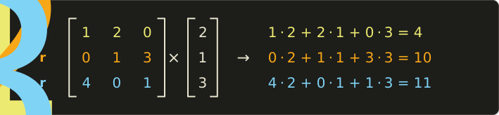
Let's do that example slowly.
Take this matrix and vector:
Row 1 is : .
Row 2 is : .
Row 3 is : .
This view is great for computing by hand: one row at a time, one dot product at a time.
It also explains the name you'll hear a lot: "a matrix is a bunch of dot products stacked on top of each other".
View 2: the result is a mix of the columns
Now let's regroup the same formula by the components of instead of by rows.
Every in the result is multiplied by something from the first column, every by something from the second column, and every by something from the third column:
If we call the columns , that's:
That's a linear combination of the columns, exactly like in chapter 2, where we wrote every vector as .
Let's check it with the same example.
The columns of are , and , and :
Same answer, , as it must be.
The key insight: columns are where the basis vectors land
Here is the single most important idea in this whole series, so I'm giving it its own section.
What happens if we multiply by the basis vector ?
We get the first column back.
In the same way, and .
So:
The first column of a matrix is where i lands. The second column is where j lands. The third column is where k lands.
And because every vector is , once you know where the three basis vectors go, you know where every vector goes: it's the same mix of the new arrows.
A matrix is a recipe: "replace i by this, j by this, k by this, and keep the same amounts".
This also explains the identity matrix.
Its columns are , and , so i lands on i, j lands on j, k lands on k.
Nothing moves, so for every vector.
A picture: transforming the unit square
Let's see this in 2D, where we can draw.
Take this matrix:
Reading its columns: lands on and lands on .
Now we transform the four corners of the unit square, the square from to :
| Corner | Calculation | Result |
|---|---|---|
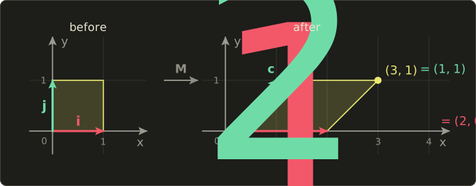
The square became a slanted parallelogram.
The bottom edge (which was ) is now twice as long, and the left edge (which was ) now leans to the right.
Every point inside the square follows along.
For example, the point goes to , and with view 1 we get the same: .
This is the trick that makes matrices readable.
When you meet a matrix in someone's code, don't stare at the numbers.
Read the columns and ask "where do i, j and k go?"
6.4 The size rule
Can you multiply any matrix with any vector?
No.
In view 1, every row is dotted with the vector, and the dot product needs two lists of the same length.
So the number of columns of the matrix must equal the number of components of the vector.
The two inner numbers must match, and the two outer numbers give the size of the result.
An m × n matrix eats an n-dimensional vector and gives back an m-dimensional vector.
The matrix doesn't have to be square.
Here is a 2 × 3 matrix that takes a 3D vector and gives a 2D vector:
Going from 3D down to 2D is exactly what has to happen when a 3D world ends up on a flat screen.
We'll do that properly (with a square 4 × 4 matrix and a trick) in chapter 12.
Trying to multiply that same 2 × 3 matrix with a 2D vector is simply undefined: row 1 has three numbers, the vector has two, there's nothing to pair the third number with.
6.5 Matrices in memory and in shaders
The math above is the same everywhere.
How a computer stores a matrix, and how each language writes it, is not.
This is the part that bites everybody at least once, so let's go slowly.
Row-major and column-major storage
Memory is a single long line of numbers, but a matrix is a grid.
So we have to pick an order.
 the matrix         row-major memory
                    (row after row)
 [ 1  2  3 ]        1 2 3 4 5 6 7 8 9
 [ 4  5  6 ]
 [ 7  8  9 ]        column-major memory
                    (column after column)
                    1 4 7 2 5 8 3 6 9
Both lines describe the same matrix.
Neither one is "correct", it's just a convention, like driving on the left or the right.
The danger is when one side writes row-major and the other side reads column-major: then the reader sees the rows as columns and gets a different matrix (the transpose, which we'll meet in chapter 7).
Our C++ Mat4 is column-major, like GLSL and OpenGL.
It stores four columns, c[0] to c[3], each one a Vec4.
Because of view 2, that's a very natural choice: c[0] is literally where the x axis lands.
When you upload a matrix from the CPU to the GPU, the shader must read it in the same order the CPU wrote it.
GLSL uniform blocks are column-major by default, which matches our Mat4 directly.
For Slang, the matrix layout used for buffers is a compiler and API setting, and we'll set it to match our C++ code in the Slang series.
HLSL is similar: the layout is a compiler option, or a row_major / column_major qualifier on the matrix.
The important rule: choose one convention and make the CPU and the shader agree.
Indexing: GLSL and Slang disagree
Here is the real trap.
GLSL and Slang both know the same math, but they index matrices differently.
- In GLSL,
m[i]is column i. Som[col][row]: column first, then row. - In Slang,
M[i]is row i. SoM[row][col]: row first, then column, like the math. - In HLSL, it's the same as Slang:
M[row][col].
The element (row 1, column 2 in math, so row 0 and column 1 in 0-based code) is written M[0][1] in Slang and HLSL but m[1][0] in GLSL.
Our C++ at() follows the math: m.at(0, 1).
The same thing happens in constructors.
When you build a matrix from a list of numbers, Slang and HLSL fill it row by row, but GLSL fills it column by column.
So the same-looking line of numbers gives a different matrix in GLSL than in Slang and HLSL.
You'll see this in the sepia example below.
Multiplying: mul in Slang, star in GLSL
In GLSL, matrix times vector is written with the normal multiplication sign: m * v.
In Slang and HLSL, you must use the function mul(M, v).
This is a classic bug.
In Slang and HLSL, * is always component-wise (element by element), even for matrices.
A * B with two float4x4 multiplies the matching elements and gives a completely different matrix, not what any transform needs.
And M * v won't give you the transformed vector either.
If your mesh vanishes or explodes after porting a shader from GLSL to Slang or HLSL, search for * next to a matrix first.
| What | Slang and HLSL | GLSL | Our C++ |
|---|---|---|---|
| Matrix types | float3x3, float4x4 |
mat3, mat4 |
Mat4 |
| Element at row r, column c | M[r][c] |
m[c][r] |
m.at(r, c) |
| Single index gives | row | column | m.c[i] is a column |
| Constructor from numbers | fills rows | fills columns | set c[0] to c[3] |
| Matrix times vector | mul(M, v) |
m * v |
m * v |
| Star between two matrices | component-wise | matrix product | matrix product (chapter 7) |
6.6 Use in graphics programming
Every vertex goes through a matrix
A 3D model is a list of vertices, and each vertex has a position stored in the model's own coordinate system.
To draw it, the vertex shader has to move every one of those positions to where it belongs on the screen.
That job is done by multiplying each position with a matrix.
Here is the smallest useful vertex shader: one 4 × 4 matrix, one multiplication.
struct Transform {
  float4x4 mvp;
};

ConstantBuffer<Transform> transform;

struct VertexOutput {
  float4 position : SV_Position;
};

[shader("vertex")]
VertexOutput vertexMain(float3 position : POSITION) {
  VertexOutput output;
  output.position = mul(transform.mvp, float4(position, 1.0));
  return output;
}
#version 450
layout(set = 0, binding = 0) uniform Transform {
mat4 mvp;
};
layout(location = 0) in vec3 position;
void main() {
gl_Position = mvp * vec4(position, 1.0);
}struct Transform {
float4x4 mvp;
};
ConstantBuffer<Transform> transform;
struct VertexOutput {
float4 position : SV_Position;
};
VertexOutput vertexMain(float3 position : POSITION) {
VertexOutput output;
output.position = mul(transform.mvp, float4(position, 1.0));
return output;
}
Notice that the 3D position is turned into a 4D vector by adding a 1.0 at the end.
That 4th number is what lets a matrix move things around, and it's the whole topic of chapter 9.
The name mvp stands for model, view and projection, three matrices we'll combine into one in chapter 7 and build in chapters 9 to 12.
For now the point is: one matrix, one mul (or *), every vertex, every frame.
The GPU runs this little program once per vertex, millions of times per frame.
A 4 × 4 matrix times a 4D vector is 16 multiplications and 12 additions, which GPUs are extremely good at.
Color matrices: grayscale and sepia
Matrices aren't only for positions.
A color is a vector too, so a 3 × 3 matrix can transform colors.
Each output channel is a dot product of one row with the input color (view 1), so each row says "how much of red, green and blue goes into this channel".
A classic grayscale filter uses the brightness weights 0.299, 0.587 and 0.114 for every channel.
Our eyes are most sensitive to green and least to blue, which is why the weights differ.
Let's apply it to orange, .
Every row is the same, so every channel gets the same value:
The result is , a medium gray.
(For grayscale alone, a single dot would do, but the matrix form lets you swap in any other filter without changing the code.)
A popular sepia filter uses three different rows:
Orange again, row by row:
So orange becomes the warm brown .
The first two rows of add up to more than 1, so pure white would become : we have to clamp the result to the 0 to 1 range.
Here it is as a shader function.
Look carefully at the constructors: the Slang and HLSL versions are written row by row, the GLSL version column by column, and all three build the same matrix .
float3 toSepia(float3 color) {
  // float3x3(...) fills row by row
  float3x3 sepia = float3x3(
    0.393, 0.769, 0.189,
    0.349, 0.686, 0.168,
    0.272, 0.534, 0.131);
  return saturate(mul(sepia, color));
}
vec3 toSepia(vec3 color) {
// mat3(...) fills column by column
mat3 sepia = mat3(
0.393, 0.349, 0.272,
0.769, 0.686, 0.534,
0.189, 0.168, 0.131);
return clamp(sepia * color, 0.0, 1.0);
}float3 toSepia(float3 color) {
// float3x3(...) fills row by row
float3x3 sepia = float3x3(
0.393, 0.769, 0.189,
0.349, 0.686, 0.168,
0.272, 0.534, 0.131);
return saturate(mul(sepia, color));
}
If you copied the Slang numbers straight into the GLSL mat3(...), you'd get a different, wrong filter, and nothing would warn you.
Photo apps, video players and post-processing stacks are full of matrices like these: saturation, hue shifts, channel swaps, color-blindness simulation.
6.7 Other uses
Matrices show up anywhere there's a table of numbers that mixes inputs into outputs.
Systems of linear equations
Remember solving two equations at school?
Put the numbers in front of and into a matrix, and the unknowns into a vector, and the whole system becomes one line:
The solution is : check it with view 1, and .
Engineers solve systems like this with thousands or millions of unknowns: bridges, circuits, weather, fluid simulation.
How to "undo" a matrix to find is chapter 10.
Markov chains
Say the weather is either sunny or rainy.
If today is sunny, tomorrow is sunny with probability 0.8 and rainy with 0.2.
If today is rainy, tomorrow is sunny with 0.4 and rainy with 0.6.
Put "from sunny" in column 1 and "from rainy" in column 2:
Today is sunny, so today's vector is .
Tomorrow: , which is just column 1, as view 2 promised.
The day after: .
The same idea drives text prediction, board-game analysis and Google's original PageRank.
Spreadsheets, images and economics
- A spreadsheet of prices (rows = shops, columns = products) times a vector of quantities gives the total bill at every shop at once: one dot product per row.
- Image editors and the web use color matrices directly: SVG has a filter called
feColorMatrix, and Android has aColorMatrixclass. - Blur and sharpen filters use small grids of numbers called kernels; they look like matrices but are applied by sliding over the image, which is a different operation.
- In economics, Leontief's input–output model describes a whole economy as a matrix: how much steel, power and labor each industry needs to produce one unit of its output.
6.8 Code
Time to add matrices to linalg.hh.
Here is the Mat4 struct, exactly as it is in the header:
// 4×4行列。列優先:c[列]が一つの列ベクトル。
// 4×4 matrix. Column-major: c[column] is one column vector.
struct Mat4 {
  Vec4 c[4];

  // 行row・列colの要素(0始まり) / element at row, col (0-based)
  float &at(int row, int col) {
    float *p = &c[col].x;
    return p[row];
  }
  float at(int row, int col) const {
    const float *p = &c[col].x;
    return p[row];
  }

  static Mat4 identity() {
    Mat4 m;
    m.c[0] = {1, 0, 0, 0};
    m.c[1] = {0, 1, 0, 0};
    m.c[2] = {0, 0, 1, 0};
    m.c[3] = {0, 0, 0, 1};
    return m;
  }
};
A few things to notice:
- The data is four
Vec4columns.m.c[0]is the first column, where the x axis lands, just likem[0]in GLSL. at(row, col)follows the math order (row first) with 0-based numbers. It finds the column, then stepsrowfloats into it. This works because the four floats of aVec4sit right next to each other in memory.- There are two versions of
at(): one returns a reference so you can writem.at(1, 2) = 3;, the other is forconstmatrices and just returns the value. identity()sets the columns to i, j, k and the 4th basis vector, so nothing moves.
And here is matrix times vector:
// 行列×ベクトル:列の線型結合 / matrix × vector: a linear combination of the columns (chapter 6)
inline Vec4 operator*(const Mat4 &m, Vec4 v) {
  return v.x * m.c[0] + v.y * m.c[1] + v.z * m.c[2] + v.w * m.c[3];
}
That one line is view 2, word for word: x times the first column, plus y times the second, plus z times the third, plus w times the fourth.
It uses the float * Vec4 and Vec4 + Vec4 operators we wrote in chapter 2.
A test program
Let's put the 3 × 3 example from section 6.3 into the top-left corner of a 4 × 4 identity matrix, and check that we get .
#include "linalg.hh"
#include <cstdio>

void printVec4(const char *name, Vec4 v) {
  printf("%s = (%g, %g, %g, %g)\n", name, v.x, v.y, v.z, v.w);
}

void printMat4(const char *name, const Mat4 &m) {
  printf("%s =\n", name);
  for (int row = 0; row < 4; ++row) {
    printf("  [%6g %6g %6g %6g ]\n", m.at(row, 0), m.at(row, 1), m.at(row, 2), m.at(row, 3));
  }
}

int main() {
  // The 3x3 example from section 6.3, inside a 4x4 identity.
  Mat4 m = Mat4::identity();
  m.at(0, 1) = 2;
  m.at(1, 2) = 3;
  m.at(2, 0) = 4;
  printMat4("m", m);

  // c[0] is the first column: where i lands.
  printVec4("m.c[0]", m.c[0]);

  Vec4 v = {2, 1, 3, 1};
  printVec4("m * v", m * v);

  // The identity matrix changes nothing.
  printVec4("I * v", Mat4::identity() * v);
  return 0;
}
Expected output:
m =
  [     1      2      0      0 ]
  [     0      1      3      0 ]
  [     4      0      1      0 ]
  [     0      0      0      1 ]
m.c[0] = (1, 0, 4, 0)
m * v = (4, 10, 11, 1)
I * v = (2, 1, 3, 1)
The printed matrix looks like the math because printMat4 walks row by row using at(), even though the memory is stored column by column.
m.c[0] prints the first column , not the first row.
The 4th component of v is 1 and the 4th column of m is , so it only adds to the w component and the first three numbers are exactly our .
6.9 Summary
- A matrix is a grid of numbers with m rows and n columns. The element is in row i, column j (1-based in math, 0-based in code).
- Matrix times vector: each output component is the dot product of one row with the vector.
- The same result is a linear combination of the columns: .
- The columns of a matrix are where the basis vectors i, j, k land. Read the columns to understand a matrix.
- The identity matrix has ones on the diagonal and changes nothing.
- An m × n matrix needs an n-vector and gives an m-vector.
- Our
Mat4is column-major like GLSL. The CPU and the shader must agree on the memory layout. - GLSL indexes
m[col][row]and its constructors fill columns. Slang and HLSL indexM[row][col]and their constructors fill rows. - In Slang and HLSL use
mul(M, v). The*operator is component-wise there, a classic porting bug.
6.10 Challenges
- ★ For , what is the size of the matrix, and what are , and ?
- ★ Compute with view 1, then again with view 2, and check that the answers match.
- ★ Without doing any row-by-row arithmetic, use the columns to compute .
- ★ Write the 2 × 2 matrix that sends i to and j to . Where does go? Draw the unit square before and after. What did the matrix do?
- ★★ Build a
Mat4by setting its columns to , , and , multiply it by and print the result. You should get(12, 15, 18, 1). Then print the matrix withprintMat4and explain why the first printed row is1 4 7 0. - ★★ Write a shader function, in both Slang and GLSL (and HLSL if you like), that swaps the red and blue channels of a color using a 3 × 3 matrix (with
mulin Slang and HLSL and*in GLSL). The color should become . Does the constructor order matter for this particular matrix? Why? - ★★★ Multiply any 3 × 3 matrix by the zero vector . What do you always get? What does that tell you about whether a 3 × 3 matrix can ever move an object from one place to another? (Chapter 9 is the answer.)
コメント(0)
まだコメントはありません。
ログインするとコメント出来ます。