9. Homogeneous Coordinates and Translation
In chapter 8 we learned how to scale, rotate, shear and mirror things with matrices.
But there is one transformation every game does thousands of times per frame that we still can't write as a matrix: simply moving something.
Moving a model from one place to another is called translation.
In this chapter I'll show you why translation doesn't fit into a 3×3 matrix, and the beautifully simple trick that makes it fit anyway: adding a fourth number called w.
This trick is called homogeneous coordinates, and it is the reason every vertex shader you'll ever write works with float4 / vec4 and 4×4 matrices.
By the end of the chapter you'll be able to build a complete model matrix that places an object anywhere in your world.
9.1 The problem: translation is not linear
Translating a point means adding the same offset to it, no matter where the point is.
If the point is and the offset is , the moved point is:
Think of sliding a cup across a table.
Every part of the cup moves by the same distance in the same direction.
Nothing turns, nothing gets bigger, nothing gets bent.
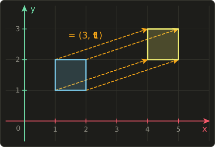
That sounds like the easiest transformation of all.
So why didn't chapter 8 include it?
Remember what chapter 8 said about linear transformations: they always keep the origin where it is.
Any matrix times the zero vector gives the zero vector, because every column gets multiplied by 0:
But translation moves the origin.
With , the origin ends up at .
So there is no 2×2 matrix (and no 3×3 matrix in 3D) that can translate.
It also breaks the other rule from chapter 8, .
If we translate the sum we add once: .
If we translate each part and then add, we get twice: .
Those are not the same, so translation is not linear.
This is a real nuisance.
We want to combine scale, rotation and translation into one matrix, so we can multiply millions of vertices by that single matrix (remember associativity from chapter 7).
If translation has to be a separate "add a vector" step, that plan falls apart.
9.2 The trick: one extra coordinate
Here is the idea: we give every point one extra coordinate that is always 1.
That extra coordinate is called w.
A 2D point becomes , and now we can use 3×3 matrices on it.
Why does that help?
Look at what a 3×3 matrix does with a vector whose last number is 1:
The third column gets multiplied by the 1 in w, so it is simply added to the result.
That's translation!
And the bottom row makes sure the result has again, so we can keep applying more matrices.
A 2D warm-up example
Let's move the point by .
First we write the point with : .
Then each output component is one row of the matrix dotted with the vector (chapter 6):
We drop the w again and read off the answer: .
That's exactly .
Why this is not cheating
It feels a bit like a magic trick, so here's a picture of what is really going on.
We put our flat 2D world on the plane , floating one unit above the origin of a 3D space.
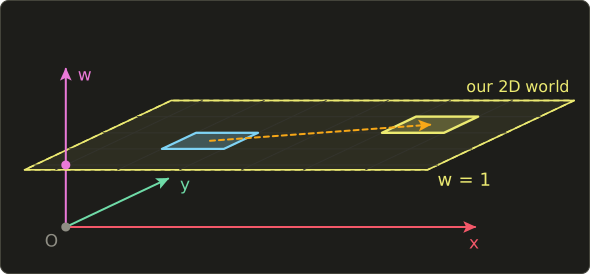
The 3×3 matrix above is a shear in that 3D space (chapter 8): it slides each layer sideways by an amount that depends on its height w.
The layer at height 1 slides by exactly .
The 3D origin (height 0) doesn't move at all, so the 3×3 matrix is still a perfectly linear transformation.
It's only our 2D world, living one floor up, that appears to be translated.
So we haven't broken any rules.
We've just moved up one dimension, where translation becomes a shear.
9.3 What the formula is
In 3D we do the same thing with four numbers: a point becomes .
These four numbers are the point's homogeneous coordinates.
The 4×4 translation matrix is:
And applying it to a point gives:
The second big rule of this chapter is about the value of w:
| Kind | w | Example | Affected by translation? |
|---|---|---|---|
| Point (a location) | 1 | a vertex position, the camera position | yes |
| Direction (an arrow) | 0 | a normal, a velocity, a light direction | no |
9.4 How it works
Worked example: moving a point
Let's move the point by .
With the point is .
Row by row:
The moved point is , which is .
Now let's look at the same calculation the other way from chapter 6: the result is a linear combination of the columns, and the weights are the components of the vector.
This view shows the whole trick very clearly.
The first three columns are the basis vectors, untouched, so x, y and z pass through unchanged.
The fourth column holds the translation, and it gets multiplied by w.
With the translation is added once.
Worked example: a direction stays put
Now take the direction with , and use the same matrix:
The fourth column was multiplied by 0, so the translation simply vanished.
The direction comes out exactly as it went in, still with .
Why directions should ignore translation
This isn't an accident, it's exactly the behavior we want.
A direction is an arrow, not a place.
It has a length and it points somewhere, but it doesn't live anywhere.
- If a car drives north at 20 m/s and I move the whole car 100 m east, it still drives north at 20 m/s. Velocity is a direction.
- If a wall faces the +X axis and I move the wall, it still faces +X. A surface normal is a direction.
- Sunlight comes from the same direction whether you stand in Tokyo or in your garden. A directional light is a direction.
Rotation and scale should still affect directions (if I turn the car, its velocity turns too), and they do, because they live in the first three columns which are multiplied by x, y and z as usual.
Only the translation column is switched off by .
Note: for normals there is one more catch when the scale is non-uniform. We'll fix that with the "normal matrix" in chapter 10.
The bookkeeping of w
The w value also keeps us honest when we do arithmetic with points and directions.
Just add or subtract the w values like any other component:
- point − point = direction, because . The arrow from A to B (chapter 2) is a direction.
- point + direction = point, because . Walking along an arrow from a place gets you to a place.
- direction + direction = direction, because .
- point + point gives , which is neither. Adding two locations has no meaning (what is "Tokyo + Paris"?).
But look at the midpoint of two points: has , a proper point.
In general a weighted sum of points is a point exactly when the weights add up to 1.
That's why lerp from chapter 2, , always gives a point: .
9.5 Affine transformations
A transformation that is "a linear transformation followed by a translation" is called an affine transformation.
Every combination of scale, rotation, shear, reflection and translation is affine.
In formula form it is:
where is a 3×3 matrix (the linear part, from chapter 8) and is the translation.
With homogeneous coordinates we can pack both into one 4×4 matrix:
The short form on the right is called a block matrix: stands for the whole upper-left 3×3 area, for the column of three numbers on the right, and for the bottom row of three zeros.
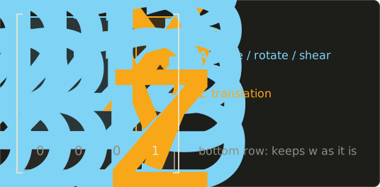
This is why the scale and rotateX / rotateY / rotateZ functions from chapter 8 already return 4×4 matrices: they are affine matrices whose is zero.
And translate is an affine matrix whose is the identity.
A very handy fact for debugging: because the fourth column, the last column of a model matrix is where the object's origin ends up in the world.
If an object shows up in the wrong place, print the last column first.
Affine transformations keep straight lines straight and parallel lines parallel, and they keep midpoints as midpoints.
What they don't keep is the origin.
And when you multiply two affine matrices, you always get another affine matrix (the bottom row stays ).
If you multiply out the blocks you get:
Read the top-right block carefully: the translation of the right matrix gets transformed by the left matrix's linear part .
That single detail explains all of the next section.
9.6 The model matrix: T R S
Every 3D model is built in its own little coordinate system, called object space or local space (chapter 11 covers all the spaces).
The artist usually puts the origin somewhere sensible: at a character's feet, at the center of a crate, at the hinge of a door.
To place the model in the world we build its model matrix from three parts:
Remember from chapter 7 that we read this right to left, because the matrix nearest to the vector acts first:
- S scales the model, around its own origin.
- R rotates the model, around its own origin.
- T moves the model to its place in the world.
The key phrase is "around its own origin".
Scaling and rotating always happen around the origin (chapter 8), so we want to do them while the model is still sitting at the origin, before we move it away.
Worked example: placing a plank
Say we have a plank model that is 1 unit long along its local X axis, and we want it 2 units long, standing upright, at position .
That's scale({2, 1, 1}), rotateZ(radians(90.0f)) and translate({5, 0, 0}).
With and the three matrices are:
Let's follow the tip of the plank, the local point , through each step:
- Scale: . The plank is now 2 long.
- Rotate 90° around Z: . The plank now points up.
- Translate: . The plank stands at x = 5.
The origin of the plank, , is not changed by S or R, and T moves it to .
That's exactly what we wanted.
We can also multiply the three matrices together once.
First (the columns of R, each scaled by the matching diagonal entry of S), then T in front:
Check: .
Same answer, but now it's a single matrix we can send to the GPU.
Notice the last column is exactly : when T is the leftmost matrix, the formula from 9.5 adds it untouched.
What goes wrong in other orders
Matrix multiplication isn't commutative (chapter 7), so other orders give other results.
Two mistakes are so common that every graphics programmer makes them at least once.
Mistake 1: translating before rotating ().
Follow the plank's origin: S does nothing, T moves it to , and then R rotates it around the world origin to .
The plank is standing at the wrong place!
In 9.5's formula, the translation became instead of .
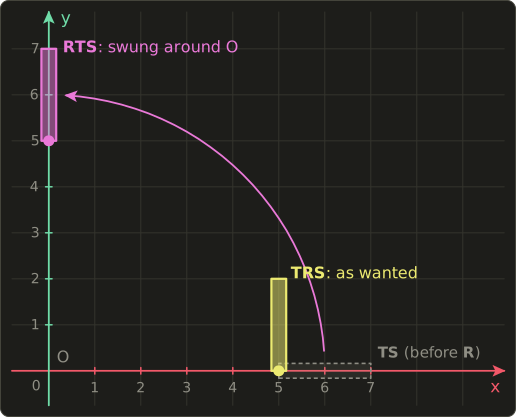
If you animate the angle, the object doesn't spin in place, it orbits around the world origin like a planet around the sun.
Sometimes that's what you want (a moon around a planet), but usually it's a bug.
Mistake 2: scaling after rotating ().
Now the plank is rotated first, so its long axis points along world Y, and only then stretched by 2 along world X.
The tip goes to , then stays , then becomes .
So the plank is still only 1 long, and it got fat instead of long.
With angles that aren't multiples of 90°, this order even turns rectangles into slanted diamond shapes, because you're stretching along a direction that is diagonal to the object.
So the rule of thumb is: T R S, read from the right: scale, then rotate, then translate.
9.7 Rotating around a pivot point
Rotations always turn around the origin.
But what if you want to rotate a door around its hinge, or a sprite around its center, when that point isn't at the origin?
The trick is a little three-step dance:
Reading right to left:
- moves everything so that the pivot sits at the origin.
- rotates around the origin, which is now the pivot.
- moves everything back.
Worked example
Let's rotate the point by 90° around the Z axis, using the pivot .
The point is 1 unit to the right of the pivot, so after a counter-clockwise quarter turn it should be 1 unit above it.
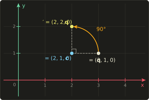
- : .
- (90° around Z sends x to y): .
- : .
The answer is , one unit above the pivot, just as the picture says.
Multiplied out, the three matrices become a single affine matrix.
Using 9.5's formula, its linear part is R and its translation is .
Here , so the translation is :
Check with : the first row gives , the second row gives .
Same .
The same dance works for scaling around a pivot: .
9.8 A peek ahead: when w is not 1
So far w has always been 1 or 0.
But what does mean?
The full rule of homogeneous coordinates is: divide everything by w to get the actual point.
So is the same point as .
Every multiple of a homogeneous vector describes the same point, which is where the word "homogeneous" comes from.
A direction with can be thought of as a "point infinitely far away" in that direction, since dividing by a smaller and smaller w sends the point further and further out.
Affine matrices never change w (their bottom row is ), so for everything in this chapter the divide does nothing.
In chapter 12 we'll meet the perspective projection matrix, which has a different bottom row and puts the distance from the camera into w.
The GPU then divides by w automatically, and that division is what makes far things look small.
That's the real reason the whole graphics pipeline works in four dimensions.
9.9 Use in graphics programming
The model matrix in the vertex shader
Every object in your scene gets its own model matrix, usually built on the CPU as translate(position) * rotation * scale(size) and uploaded as a uniform.
The vertex shader then turns each vertex position into a float4 with , and each normal into a float4 with .
Here's a minimal vertex shader that does exactly that.
The view and projection matrices (view, proj) are covered in chapters 11 and 12; for now, just treat them as "the camera".
struct Matrices {
  float4x4 model;
  float4x4 view;
  float4x4 proj;
};
ConstantBuffer<Matrices> matrices;

struct VSInput {
  float3 position : POSITION;
  float3 normal   : NORMAL;
};

struct VSOutput {
  float4 position    : SV_Position;
  float3 worldNormal : NORMAL;
};

[shader("vertex")]
VSOutput vertexMain(VSInput input) {
  VSOutput output;
  // Point: w = 1, so the translation is applied
  float4 worldPos = mul(matrices.model, float4(input.position, 1.0));
  output.position = mul(matrices.proj, mul(matrices.view, worldPos));
  // Direction: w = 0, so the translation is ignored
  output.worldNormal = mul(matrices.model, float4(input.normal, 0.0)).xyz;
  return output;
}
#version 450
layout(set = 0, binding = 0) uniform Matrices {
mat4 model;
mat4 view;
mat4 proj;
};
layout(location = 0) in vec3 inPosition;
layout(location = 1) in vec3 inNormal;
layout(location = 0) out vec3 worldNormal;
void main() {
// Point: w = 1, so the translation is applied
vec4 worldPos = model * vec4(inPosition, 1.0);
gl_Position = proj * (view * worldPos);
// Direction: w = 0, so the translation is ignored
worldNormal = (model * vec4(inNormal, 0.0)).xyz;
}struct Matrices {
float4x4 model;
float4x4 view;
float4x4 proj;
};
ConstantBuffer<Matrices> matrices;
struct VSInput {
float3 position : POSITION;
float3 normal : NORMAL;
};
struct VSOutput {
float4 position : SV_Position;
float3 worldNormal : NORMAL;
};
VSOutput vertexMain(VSInput input) {
VSOutput output;
// Point: w = 1, so the translation is applied
float4 worldPos = mul(matrices.model, float4(input.position, 1.0));
output.position = mul(matrices.proj, mul(matrices.view, worldPos));
// Direction: w = 0, so the translation is ignored
output.worldNormal = mul(matrices.model, float4(input.normal, 0.0)).xyz;
return output;
}
A classic bug is to write float4(input.normal, 1.0) by copy-paste.
Then every normal gets the object's position added to it, and the lighting goes completely wrong as soon as the object moves away from the origin.
If your lighting looks fine at the origin but breaks when you move the object, check the w of your normals first.
Placing many instances
A forest doesn't need a thousand tree models.
It needs one tree model and a thousand model matrices.
On the CPU it looks like this:
for (int i = 0; i < 3; ++i) {
  float height = 1.0f + 0.5f * i;
  Mat4 model = translate({3.0f * i, 0.0f, 0.0f}) * rotateY(0.7f * i) * scale({1.0f, height, 1.0f});
  Vec4 top = model * Vec4{0.0f, 2.0f, 0.0f, 1.0f};
  printf("tree %d top: (%.2f, %.2f, %.2f)\n", i, top.x, top.y, top.z);
}
tree 0 top: (0.00, 2.00, 0.00)
tree 1 top: (3.00, 3.00, 0.00)
tree 2 top: (6.00, 4.00, 0.00)
Each tree gets a different position, rotation and height, and the top of the tree (local point ) lands in a different place.
With instanced rendering you put all those matrices into one buffer and draw the tree once with an instance count; the shader picks its matrix with the instance index:
StructuredBuffer<float4x4> instanceModels;

[shader("vertex")]
float4 instancedMain(float3 position : POSITION, uint instanceId : SV_InstanceID) : SV_Position {
  float4x4 model = instanceModels[instanceId];
  return mul(model, float4(position, 1.0));
}
#version 450
layout(std430, set = 0, binding = 1) readonly buffer Instances {
mat4 instanceModels[];
};
layout(location = 0) in vec3 inPosition;
void main() {
mat4 model = instanceModels[gl_InstanceIndex];
gl_Position = model * vec4(inPosition, 1.0);
}StructuredBuffer<float4x4> instanceModels;
float4 instancedMain(float3 position : POSITION, uint instanceId : SV_InstanceID) : SV_Position {
float4x4 model = instanceModels[instanceId];
return mul(model, float4(position, 1.0));
}(To keep it short this example stops at world space; a real one would multiply by view and projection as above.)
Parent-child transforms
In chapter 7 we saw that a child's world matrix is its parent's world matrix times its own local matrix.
Now we can make that concrete, because local matrices can include translation.
A sword in a hand is handWorld * swordLocal, where swordLocal might be translate({0.0f, 0.1f, 0.0f}) * rotateX(angle): "a little above the hand's origin, tilted by some angle".
A wheel on a car is carWorld * translate(wheelOffset) * rotateX(spin).
When the car moves, the wheel follows automatically, and the wheel still spins around its own axle because its rotation sits to the right of its translation, exactly the T R S rule again.
2D sprites and UI with 3×3 matrices
For 2D games and user interfaces we only need the warm-up version from 9.2: 3×3 matrices and float3(x, y, 1.0).
A sprite's transform is again , just in 2D, and rotating a button around its center uses the pivot trick from 9.7.
float2 transformPoint2D(float3x3 m, float2 p) {
  return mul(m, float3(p, 1.0)).xy;
}

float2 transformDirection2D(float3x3 m, float2 d) {
  return mul(m, float3(d, 0.0)).xy;
}
vec2 transformPoint2D(mat3 m, vec2 p) {
return (m * vec3(p, 1.0)).xy;
}
vec2 transformDirection2D(mat3 m, vec2 d) {
return (m * vec3(d, 0.0)).xy;
}float2 transformPoint2D(float3x3 m, float2 p) {
return mul(m, float3(p, 1.0)).xy;
}
float2 transformDirection2D(float3x3 m, float2 d) {
return mul(m, float3(d, 0.0)).xy;
}
Tip: in uniform and storage buffers, each column of a 3×3 matrix is padded to the size of four floats. Many engines therefore send 2D transforms as a 4×4 matrix (or three float4 values) to avoid layout surprises.
9.10 Other uses
Homogeneous coordinates and 4×4 affine matrices aren't just a graphics thing:
- Robotics: a robot arm is a chain of joints, and each joint's position and orientation relative to the previous one is a 4×4 homogeneous transform (the Denavit–Hartenberg convention is a standard recipe for building them). Multiplying the chain gives the position of the gripper.
- CAD assemblies: every part of a machine is placed inside its sub-assembly with a 4×4 matrix, and every sub-assembly inside the main assembly with another one, exactly like a scene graph.
- Image editing and computer vision: an affine image warp (rotate, scale, skew and shift a photo) uses the top two rows of a 3×3 homogeneous matrix. OpenCV's
warpAffinetakes exactly that 2×3 matrix. - Vector graphics: SVG's
matrix(a, b, c, d, e, f), PDF and the HTML canvastransformmethod all use the same six numbers: a 2×2 linear part plus a translation. - GIS and maps: a georeferenced satellite image stores six numbers (a so-called geotransform or world file) that map pixel coordinates to map coordinates, which is a 2D affine transform once again.
9.11 Code
Here's this chapter's addition to linalg.hh.
It's short, because all the work is in the structure of the matrix: start with the identity and replace the fourth column (c[3], remember our Mat4 stores columns) with .
// 平行移動 / translation (chapter 9)
inline Mat4 translate(Vec3 t) {
  Mat4 m = Mat4::identity();
  m.c[3] = {t.x, t.y, t.z, 1.0f};
  return m;
}
And here's a test program that repeats every worked example from this chapter.
I use radians() from chapter 1 for the angles.
Because cos(radians(90.0f)) isn't exactly 0 in floating-point math (it's about −0.00000004), I added a tiny tidy helper so the output doesn't show ugly -0.00 values.
#include "linalg.hh"
#include <cstdio>

// 浮動小数点の-0.00を避ける / avoid printing -0.00
static float tidy(float v) { return std::fabs(v) < 1e-5f ? 0.0f : v; }

static void print(const char *name, Vec4 v) {
  printf("%-10s (%.2f, %.2f, %.2f, %.2f)\n", name, tidy(v.x), tidy(v.y), tidy(v.z), tidy(v.w));
}

int main() {
  // 1. Translation alone
  Mat4 t = translate({4.0f, -1.0f, 2.0f});
  print("point", t * Vec4{1.0f, 2.0f, 3.0f, 1.0f});
  print("direction", t * Vec4{1.0f, 2.0f, 3.0f, 0.0f});

  // 2. A model matrix: scale, then rotate, then translate
  Mat4 model = translate({5.0f, 0.0f, 0.0f}) * rotateZ(radians(90.0f)) * scale({2.0f, 1.0f, 1.0f});
  print("tip", model * Vec4{1.0f, 0.0f, 0.0f, 1.0f});
  print("origin", model * Vec4{0.0f, 0.0f, 0.0f, 1.0f});
  print("axis", model * Vec4{1.0f, 0.0f, 0.0f, 0.0f});

  // 3. The wrong order: translate first, then rotate
  Mat4 orbit = rotateZ(radians(90.0f)) * translate({5.0f, 0.0f, 0.0f}) * scale({2.0f, 1.0f, 1.0f});
  print("orbit", orbit * Vec4{0.0f, 0.0f, 0.0f, 1.0f});

  // 4. Rotating around a pivot point
  Vec3 pivot{2.0f, 1.0f, 0.0f};
  Mat4 aroundPivot = translate(pivot) * rotateZ(radians(90.0f)) * translate(-pivot);
  print("pivot", aroundPivot * Vec4{3.0f, 1.0f, 0.0f, 1.0f});
  return 0;
}
Expected output:
point      (5.00, 1.00, 5.00, 1.00)
direction  (1.00, 2.00, 3.00, 0.00)
tip        (5.00, 2.00, 0.00, 1.00)
origin     (5.00, 0.00, 0.00, 1.00)
axis       (0.00, 2.00, 0.00, 0.00)
orbit      (0.00, 5.00, 0.00, 1.00)
pivot      (2.00, 2.00, 0.00, 1.00)
Look at the "axis" line: the direction was scaled and rotated into , but not moved to x = 5.
That's doing its job.
9.12 Summary
- Translation moves the origin, so it is not linear and can't be a 3×3 matrix.
- Homogeneous coordinates add a fourth number w. Points use , directions use .
- The 4×4 translation matrix is the identity with in the last column, which gets multiplied by w.
- Directions (normals, velocities, light directions) ignore translation automatically because their w is 0.
- Affine transformation = linear part plus translation: . The last column of a model matrix is the object's position.
- The model matrix is : scale, then rotate, then translate. Other orders cause orbiting or stretching along the wrong axis.
- Rotating around a pivot: .
- The general rule is to divide by w. That becomes important for perspective in chapter 12.
9.13 Challenges
- ★ Write the 4×4 matrix and apply it to the point , row by row. You should get . Then apply it to the direction : what comes out, and what is its w?
- ★ In 2D with 3×3 matrices, compute as one matrix and apply it to the point . You should get .
- ★ In 2D, apply both and to the point . One gives and the other . Which order "orbits", and why?
- ★ Rotate the 2D point by 90° counter-clockwise around the pivot using the three steps from 9.7. You should get .
- ★★ Write
Vec3 transformPoint(const Mat4 &m, Vec3 p)andVec3 transformDirection(const Mat4 &m, Vec3 d)(w = 1 and w = 0). Fortranslate({1, 2, 3}) * scale({2, 2, 2}), the point should give and the direction should give . - ★★ Write
Mat4 rotateYAround(Vec3 pivot, float angle)using the pivot trick androtateY. Rotating by 90° around the pivot should print(1.00, 0.00, -1.00). - ★★★ Multiply out in general. What do you get, and does the order matter? Then use 9.5's block formula to explain why has the translation , and when that translation is zero.
コメント(0)
まだコメントはありません。
ログインするとコメント出来ます。